Mass Source Definition
In ETABS, the user has the option of choosing one of three options for defining the
source of the mass of a structure. Click the Define menu -> Mass Source command to
bring up the Define Mass Source form. The following options appear on the form:
1. From Self and Specified Mass:
Each structural element has a material property associated with it; one of
the items specified in the material properties is a mass per unit volume.
When the ‘From Self and Specified Mass’ box is checked, ETABS
determines the building mass associated with the element mass by
multiplying the volume of each structural element times it’s specified
mass per unit volume.
2. From Loads:
This specifies a load combination that defines the mass of the structure.
The mass is equal to the weight defined by the load combination divided
by the gravitational multiplier, g. This mass is applied to each joint in the
structure on a tributary area basis in all three translational directions.
3. From Self and Specified Mass and Loads:
This option combines the first two options, allowing you to consider self-
weight, specified mass, and loads in the same analysis.
It is important to remember when using the ‘From Self and Specified Mass and
Loads’ option, NOT to include the Dead Load Case in the ‘Define Mass Multiplier
for Loads’ box. This will account for the dead load of the structure TWICE.
For this example, we will choose the first option ‘From Self and Specified Mass’.
Time History Load Application
In this example, we are interested in defining a pre-defined time history function from a
text file. Go to Define>Time History Function>Add Function from File. Click the
Browse button and select the time history text file. The record we have selected is the
1940 El Centro earthquake record. This text file contains time and acceleration values for
the specified earthquake. You can view time history graph by clicking on the Display
Graph button. Fill in the Function File information:
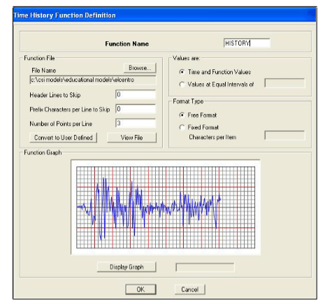
Figure 20 Time History Function Definition
Next, we define the Time History case data. Go to Define->Time History Cases-> Add
New History. There are many options available including Analysis Type, Number of
Output Time Steps and Output Time Step Size. The output time step size is the time in
seconds between each of the equally spaced output time steps. Do not confuse this with
the time step size in your input time history function. The number of output time step size
can be different from the input time step size in your input time history function. The
number of output time steps multiplied by the output time step size is equal to the length
of time over which output results are reported.
We are interested in assigning the time history acceleration in the x-direction. The time
history is a 12-second record, so enter 6000 time steps and time step size of .002 seconds.
Enter a scale factor of 386.4 if you are using k-in units. Please see Figure 21:
Figure 21 Time History Case Definition
It is now time to run the analysis. First, go to Analyze>Set Analysis Options>click on Set
Dynamic Parameters. You will see that by default there are 12 mode shapes that will be
calculated. Change this value to 36 mode shapes and click OK. Go to Analyze>Run
Analysis and the model will complete the analysis.