
Dynamic Charting
When you’re creating charts in financial models or reports, you should still follow best practice and try to make your models as flexible and dynamic as you can. You should always link as much as possible in your models, and this goes for charts as well. It makes sense that when you change one of the inputs to your model, this should be reflected in the chart data, as well as the titles and labels.
Building the chart on formula-driven data
Take a look at the five-year strategic forecast model that you work on in the “Conveying Your Message by Charting Scenarios” section at the beginning of this chapter. Because the chart you built was based on formulas, the chart will auto- matically change when the drop-down box is changed. Download File 0901.xlsx from www.dummies.com/go/financialmodelinginexcelfd. Open it and select the tab labeled 9-23 to try it out for yourself, as shown in Figure 9-23.
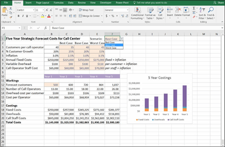
Changing the drop-down box.
 If you hide data in your source sheet, it won’t show on the chart. Test this by hid- ing one of the columns on the Financials sheet and check that the month has disappeared on the chart. You can change the options under Select Data Source so that it displays hidden cells.
Linking the chart titles to formulas
Because all the data is linked to the drop-down box, you can easily create a dynamic title in the chart by creating a formula for the title and then linking that title to the chart. Follow these steps:
-
In cell A1 of this model, change the title to the following: =“Five Year Strategic Forecast Costs for Call Center – “&F1.
 The ampersand (&) serves as a connector that will string text and values from formulas together.
 Instead of the ampersand, you can also use the CONCATENATE function, which works very similarly by joining singular cells together, or the TEXTJOIN function is a new addition to Excel 2016, which will join together large quantities of data.
When you have the formula in cell A1 working, you need to link the title in the chart to cell A1.
-
Click the title of the chart.
This part can be tricky. Make sure you’ve only selected the chart title.
-
Click the formula bar.
-
Type = and then click cell A1, as shown in Figure 9-24.
-
Press Enter.
The chart title changes to show what is in cell A1.
 You can’t insert any formulas into a chart. You can only link a single cell to it. All calculations need to be done in one cell and then linked to the title as shown.

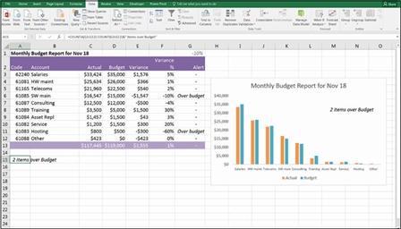
Take a look at the monthly budget report shown in Figure 9-25. We’ve already built formulas in columns F and G, which will automatically update as the data changes, and display how we’re going compared to budget. (To see how to build this model, turn to Chapter 7.)
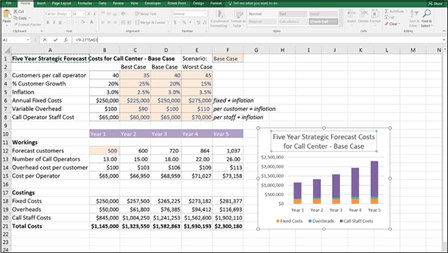 FIGURE 9-24:
Linking the chart titles to formulas.
Now you’ll create a chart based on this data, and every time the numbers change, you’ll like to be able to see how many line items are over budget. Follow these steps:
- Highlight the data showing the account, actual, and budget values in columns B, C, and D, respectively.
- Select the fi 2-D Column option from the Charts section of the Insert tab on the Ribbon to create a clustered column chart, as shown in Figure 9-25.
- In cell A1, create a heading with a dynamic date (as described in the “Using dynamic dates” sidebar).
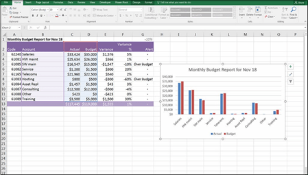 FIGURE 9-25:
Creating a clustered column chart.
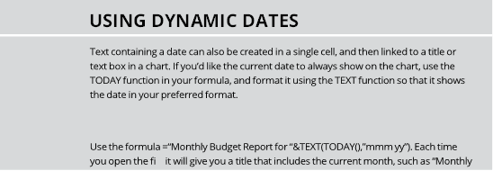
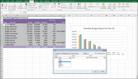 FIGURE 9-26:
Sorting the chart data.
-
Link the title of the chart to the formula in cell A1, as shown in the
preceding section.
-
Edit the chart so that the titles are horizontally aligned and change the colors.
This chart will look much better if it’s sorted so that the larger bars are on the left side.
-
Highlight all the data including the headings, and click the Sort button (in the Sort & Filter section of the Data tab in the Ribbon).
The Sort dialog box appears.
-
Sort by Actual from largest to smallest, as shown in Figure 9-26.
It’s very easy to mess up formulas when sorting, so be sure that you highlight all the columns from columns A to G before applying the sort.
Now, add some text commentary to the chart. You can do this by adding commentary in a single cell, which is dynamically linked to values in the model and link the cell to a text box to show the commentary on the chart.
-
In cell A15, create a formula that will automatically calculate how many
line items are over budget.
You can do this with the formula =COUNTA(G3:G12)-COUNT(G3:G12), which calculates how many non-blank cells are in column G. (For more information on how the COUNTA and COUNT functions work, see Chapter 7.)
- You can see that two line items are over budget, so convert this to dynamic text with the formula =COUNTA(G3:G12)-COUNT(G3:G12)&” Items over Budget” (see Figure 9-27).
FIGURE 9-27:
Completed chart with dynamic
text box.
-
Insert a text box into the chart by pressing the Text Box button in the
Text group on the Insert tab in the Ribbon.
-
Click the chart once.
The text box appears.
- Carefully select the outside of the text box with the mouse, just as you did in the last section when linking the chart titles.
- Now go to the formula bar and type =.
- Click cell A15 and click Enter.
- Resize and reposition the text box as necessary.
-
Test the model by changing the numbers so that more items are over
budget, and make sure that the commentary in the text box changes.
Charting is an important part of the final stage of the model-building process. Make sure that the key messages from the model’s output are accurately pre- sented by using clear, attractive, and unambiguous charts and tables.
Data visualization is a discipline that is increasingly growing in popularity, and not one that comes naturally to many with an analytical background — like me! Although I readily admit that it doesn’t come naturally to me, I’ve spent a lot of time learning about these principles to improve the models and dashboards that I build for clients. If you can educate yourself on even the most basic principles of visual design and apply them to your work, you and your financial models will have greater credibility and recognition in your organization and amongst your peers.


