
Calculating Expenses
Now that you’ve projected your revenue, it’s time to project your expenses for the business.
Your assumption for the barista’s annual salary is $50,000, so your annual pro- jection should be divided by the 12 months of the year to arrive at the monthly amount. Follow these steps:
- Go to the Expenses worksheet and select cell D5.
- Enter the formula =Assumptions!$B$20 and then press F4 to lock the reference.
- Enter /12 in order to divide the annual salary by 12 months.
-
Press Enter to complete the formula.
The formula will be =Assumptions!$B$20/12. The calculated result is $4,167.
-
Copy this formula across the row to calculate this for the entire year.
You’ve also assumed that it will cost an extra 25 percent of the barista’s salary to cover other staff costs and benefi Calculate this amount next.
- On the Expenses worksheet in cell D6 enter the formula
=D5*Assumptions!$B$21.
The calculated result is $1,042.
- Copy this formula across the row to calculate this for the entire year.

Your staff costs should total $5,208 every month of the year, shown in row 7.
Now you need to calculate your other costs, like rent and utilities. Follow these steps, starting with rent, which has a base case assumption of $1,200 per month:
-
On the Expenses worksheet, select cell D9, enter the formula
=Assumptions!$B$23, and press F4 to lock the reference.
The calculated result for rent is $1,200.
-
Copy this formula across the row to calculate this for the entire year.
Your assumption for utilities is $100 per month.
-
On the Expenses worksheet, select cell D10, enter the formula
=Assumptions!$B$24, and press F4 to lock the reference.
The calculated result for utilities is $100.
-
Copy this formula across the row to calculate this for the entire year
Your assumption for consumables expenses is an average of $0.45 per cup. You need to multiply this amount by the number of cups sold per month. You haven’t calculated the number of cups sold per month, so you need to do this in the formula, too.
- On the Expenses worksheet, select cell D11 and enter =Revenue!B8*Assum ptions!B32*Assumptions!$B$17.
This formula multiplies
- The number of cups sold per day in January on the Revenue worksheet in cell B8
- The number of business days in January on the Assumptions worksheet in
- The number of cups sold per day in January on the Revenue worksheet in cell B8
cell B32
- The cost of consumables per cup on the Assumptions worksheet in cell B17
The calculated result is $950.
Note that only the reference for the consumables per cup needs to be anchored as an absolute reference, because the other references need to change as you copy the formula across the row.
-
Copy this formula across the row to calculate this for the entire year.
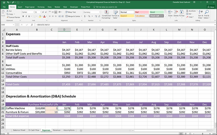
Your costs should total $7,459 for January. You’ve just projected your cash expenses for the business! Check your totals against Figure 10-6.
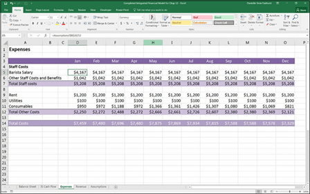 FIGURE 10-6:
Completed expense calculations.
Depreciation and amortization (D&A) expenses are non-cash expenses used in accounting. They represent the cost of a long-term fixed asset, like property, plant, and equipment (PP&E), that is steadily allocated as an expense over the useful life of the asset. Because the business is generating revenue from this asset over an extended period of time, it makes sense to apportion the expense over the period of time for which it is going to be used.
So, for example, the coffee machine will cost you $10,000 and you expect it to last for three years. From an accounting perspective, it wouldn’t be accurate to put the entire amount in the expenses on the income statement for the first month of operation because your income statement would show that you’d be making a huge loss in the first month and a huge profit thereafter. It makes more sense to
spread the cost across the entire life of the assets because that will accurately reflect the costs of purchasing the coffee machine.
 Amortization refers to the depreciation of intangible or nonphysical assets the company might hold on its balance sheet, such as goodwill, trademarks, or pat- ents. For this example, your business only holds tangible assets so you only need to calculate the depreciation, not amortization.
When you decide that a large item of expenditure is an asset, rather than an oper- ating expense, you need to put the cost of the asset onto the balance sheet and begin to depreciate it, which will be shown on the income statement. When you do this, the balance sheet changes as does the profitability shown on the income statement. The cash flow statement remains unchanged (because you need to pay for the item in any case). The process of taking a large item of expenditure and putting it onto the balance sheet rather than showing it on the income statement is called capitalization.

 When you capitalize an asset, the ongoing depreciation on the income statement affects the business’s taxable income; there are all sorts of accounting rules and regulations that differ between regions about how large an asset needs to be before it can be capitalized and over how many years it should be depreciated.
The most common method of depreciation is the straight-line method, which means that the asset is depreciated equally over its useful life. For more informa- tion on other methods of depreciation and how to calculate them in Excel, see Chapter 9 of my book Using Excel for Business Analysis: A Guide to Financial Modelling Fundamentals, Edition Revised for Excel 2013 (Wiley).
You’re going to make the assumption that your coffee machine ($10,000) will be depreciated over three years, and the furniture and fixtures ($35,000) will be depreciated over ten years. Using the straight-line method, you can calculate the depreciation simply by dividing the cost of the asset by the number of years. You need to enter this amount into the model to determine its depreciation.
You’ve already entered the capital costs on the Uses of Funds section on the bal- ance sheet, so you can reference these numbers to build your depreciation sched- ule. Follow these steps:
- On the Expenses worksheet, enter the useful life of the coff machine (3 years) in cell C20 and the useful life of the furniture and fi (10 years) in cell C21, as shown in Figure 10-7.
-
Select cell B20 and enter the formula =’Balance sheet’!K11.
This formula links this cell to the purchase price of the coff machine on the Balance Sheet worksheet. The calculated result is $10,000.
-
Select cell B21 and enter the formula =’Balance sheet’!K12.
This formula links this cell to the assumed furniture and fi es amount on the Balance Sheet worksheet. The calculated result is $35,000.
Finally, you have to fi out the monthly depreciation and amortization expense using the straight-line method. This is done by dividing the cost of the long-term asset by its useful life to fi the annual depreciation expense, and then dividing by 12 to fi the monthly expense.
-
In cell D20, enter =B20/C20/12.
 This formula divides the price of the coff machine ($10,000) by the useful life (3 years) and then converts it to monthly by dividing it by 12. The calculated result is $278. Don’t worry about the cell referencing just yet.
 Although fi modeling best practice tells you to never hard-code a number into a formula, entering 12 for the number of months is okay because it’s not a variable that is likely to change in the near future!
Because you can copy this formula down to the next row as well as across the page, you can save time by making use of mixed cell referencing.
-
Go back into your formula in cell D20 and add a dollar sign before the column referencing; the formula should now be =$B20/$C20/12.
You can do this by manually typing it in, or click within each cell reference and
press the F4 shortcut key three times. The calculated result is still $278.
- Copy this formula across the row as well as down to row 21 to calculate the depreciation for both assets for the entire year.
-
Add the sum total in row 22 using the formula =SUM(D20:D21) and copy it across the entire row.
The calculated result for each month is $569.
You’ve just projected your depreciation costs for the business. Check your totals against Figure 10-7.
FIGURE 10-7:
Completed expenses including depreciation and amortization.


