Financial Modeling in Excel Calculating Revenue

April 22, 2023

16 Views 0

SaveSavedRemoved 0

Calculating Revenue

Now that you’re happy with your assumptions, you can use them to calculate the revenue of the business for the next year.

Projecting sales volume

You know that your base case assumption is that the cafe will sell 120 cups of coffee per day, so you need to multiply this assumption by the monthly seasonal- ity to arrive at the number of cups sold per day in each month. Follow these steps:

Go to the Revenue worksheet and select cell B5.

In this cell, you’re going to enter a formula to calculate the total number of cups of coff
Type =.
Go to the Assumptions worksheet and select cell B9.
Press F4 to lock the reference.

You need to anchor this reference because as you copy the formula across, you don’t want B9 to change to another cell. For more information about cell referencing, see Chapter 6.
Stay on the Assumptions worksheet and multiply this reference by the monthly seasonality assumption by typing * and selecting cell B34.

There is no need to anchor the seasonality reference because you want the

reference to change as you copy it along the row.
Press Enter to fi the formula.

Your formula will look like this: =Assumptions!$B$9*Assumptions!B34. The calculated result is 96.
Copy this formula across the row by selecting cell B5, pressing Ctrl+C, selecting cells C5 through M5, and pressing Ctrl+V or Enter.

You have the total number of cups sold per day. Now you need to project how many of these cups are large and how many are small based on your assumptions. You’re going to use the calculated value of 96 and split it into large and small cups, based on your assumed split between large and small on the Assumptions worksheet. Follow these steps:

On the Revenue worksheet, select cell B6 and type =.
Go to the Assumptions worksheet, select cell B12, and press F4 to lock the reference.
Multiply this value by typing *.
Go back to the Revenue worksheet and select cell B5.
Press Enter to fi the formula.

Your formula will look like this: =Assumptions!$B$12*Revenue!B5. The calculated result is 38.
Copy this formula across the row to calculate this for the entire year.

You’re going to repeat this process to fi the number of small cups.
On the Revenue worksheet, select cell B7 and type =.
Go to the Assumptions worksheet, select cell B13, and press F4 to lock the reference.
Multiply this value by typing *.
Go back to the Revenue worksheet and select cell B5.

Your formula will look like this: =Assumptions!$B$13*Revenue!B5. The calculated result is 58.
Copy this formula across the row to calculate this for the entire year.
On the Revenue worksheet, select cell B8 and enter the formula

=SUM(B6:B7).

If you prefer, you can use the AutoSum function or the shortcut Alt+=. The

calculated result is 96.
Copy this formula across the row to calculate this for the entire year.
Perform a sense-check by highlighting both cells B6 and B7.

If you look at the status bar, the SUM will equal 96, the total number of cups sold per day.

Go one step further than sense-checking and add an error check in row 9.
In cell B9, enter the formula =B8-B5 and copy it across the row.

Always sense-check your numbers as you build a model. Don’t leave it to the end to check your numbers. Never take the number given for granted. Work it out in your head and use a calculator to make sure your numbers look right. This will help you make sure the numbers you’ve calculated are correct. When you’re sure the numbers are right, add in an error check if you can just like you did in row 9. A good financial modeler is always looking for opportunities to put error checks into their models. For more information about error checks, see Chapters 6 and 13.

Projecting dollar sales

Now that you’ve projected how many cups and sizes you’ll sell per day in each month, it’s time to translate this into actual dollar sales figures. Follow these steps:

On the Revenue worksheet, select cell B12 and multiply B6 (the number of large cups sold per day in January) by the price per large cup with the formula =B6*Assumptions!$C$12.

The calculated result is $154.
Copy this formula across the row to calculate this for the entire year.
On the Revenue worksheet, select cell B13 and multiply B7 (the number of small cups sold per day in January) by the price per small cup with the formula =B7*Assumptions!$C$13.

The calculated result is $202.
Copy this formula across the row to calculate this for the entire year.
Add the sum total in cell B14 with the formula =SUM(B12:B13) The calculated result is $355.
Copy this formula across the row to calculate this for the entire year.

You now have sales per day fi for large cups, small cups, and total cups for each given month. In order to fi each month’s total sales, you must multiply daily sales by the number of business days per month.
On the Revenue worksheet, select cell B15 and multiply the daily sales fi in cell B14 by the number of business days in January with the formula =B14*Assumptions!B32.

Note that you don’t need to press F4 to add any cell referencing because you

want the cell references to copy across. The calculated result is $7,814.
Copy this formula across the row to calculate this for the entire year.

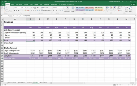
You’ve now projected your monthly sales for the year! Check your totals against Figure 10-5.