
Financial Modeling in Excel Applying Sensitivity Analysis with Data Tables
Applying Sensitivity Analysis with Data Tables
Data tables are among the more advanced and complex financial modeling tools available. Data tables can be used for scenarios and sensitivity analysis, but they’re less commonly used because they’re more advanced. Data tables are unlike most other formulas in that you can’t trace dependents, and they’re very difficult to follow unless you’re familiar with them. If anyone you work with doesn’t know data tables, he won’t be able to edit the table or make any changes.
Let’s go back to the profitability model you created in Chapter 6. I recommend that you work through the internal links exercise in Chapter 6, or download the completed version of this model, called File 0603.xlsx, from www.dummies.com/
go/financialmodelinginexcelfd
first so that you understand how this simple model works before adding sensitivities to it.
Because the model links directly to assumptions, you can use data tables to test the sensitivity of the profit margin to changes in assumptions such as the number of units sold and the cost per unit.
The existing model has a simple Income Statement linking to a number of input variables. You can test the sensitivity of one of the outputs, such as the profit margin, to variations in the input variables. Let’s see how much the profit margin changes when the sales price and cost per unit inputs change. Of course, you could do this manually, but to see the various outputs in a single table, you need to use a data table.
Building a data table with one input
To create a data table in this model, follow these steps:
-
Download File 0802.xlsx from www.dummies.com/go/financialmodeling inexcelfd, open the fi and select the Assumptions tab.
You’re testing how sensitive the profi margin is to changes in the sales price. The inputs for the sales price to be used in the data table have been entered in column A already. The next thing you need to do is to link the output cell to the data table. This needs to go at the top of the data table.
-
Link cell B9 to the profi margin using the formula =‘Summary’!B9.
Don’t type this in — press = and then click the Summary tab, select cell B9, and
press Enter.
-
Highlight the entire data table in cells A9:B15, including the output cell, as shown in Figure 8-6.
Note that you must highlight all these cells in order for it to work.
-
Select What-if Analysis from the Data tab and choose Data Table from the options (refer to Figure 8-6).
The Data Table dialog box appears.
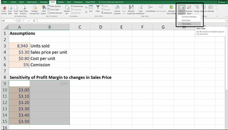
Selecting the Data Table tool on the
Ribbon.
Because you’re only doing a one-input data table, you only need to enter data for one variable, but which variable depends on how the data table is arranged and whether the input variable you’re testing is in a row or a column. Because it’s in a column, you should use the Column input cell fi
-
Link the column input cell fi to the input fi for the sales price (cell
A4) as shown in Figure 8-7.
-
Click OK.
Your data table populates with the completed sensitivity table, as shown in
Figure 8-8.
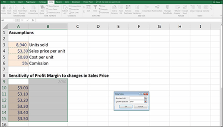 FIGURE 8-7:
Linking the one input data table to the input cell.
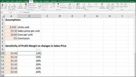 FIGURE 8-8:
Completed one-input data table.
Note that the formulas in the data table will have curly brackets around them like this =TABLE{,A4}. This is because it’s an array formula. Array formulas work dif- ferently from ordinary formulas because array formulas treat the data like an array instead of a single data value. For this reason, you can’t edit or delete a single cell within a data table in isolation. To make any changes, you need to use the Data Table tool or highlight all the formulas from cell A10 to B15, press Delete, and start again.
Building a data table with two inputs
You can add another input to your data table by listing another input variable across the top. Let’s add the cost per unit as well as the sales price, and this time, we’ll test the total profit (the dollar value) instead of the profit margin (percent- age). To complete this sensitivity analysis, follow these steps:
-
Scroll down the model to cell A18 and link it to the total profi using the
formula =‘Summary’!B8.
-
Highlight the entire data table in cells A18:E24, including the output cell, as shown in Figure 8-9.
Note that again, you must highlight all these cells in order for it to work.
-
Select What-if Analysis from the Data tab and choose Data Table from the options.
The Data Table dialog box appears.
-
Link the row input cell fi to the input fi for the cost per unit (A5)
and the column fi to the input fi for the sales price (A4), as shown in
Figure 8-9.
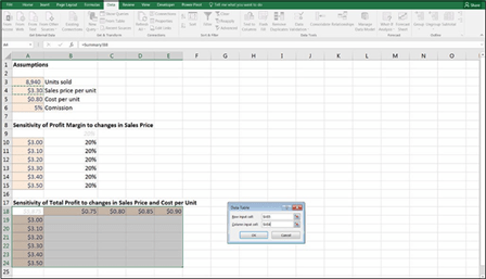 FIGURE 8-9:
Linking the two-input data table to the input cells.
-
Click OK.
Your data table populates with the completed sensitivity table, as shown in
Figure 8-10.
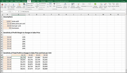 FIGURE 8-10:
Completed two-input data table.
Applying probability weightings to your data table
The great thing about adding a data table to your financial model is that it gives you a large number of variables. However, you know that only one of these can be correct! You can try to reduce the amount of uncertainty by adding probability weightings to a data table because you know that not all outcomes are equally likely.

 If you believe certain outcomes to be equally likely, then use the same weighting, while still retaining the probability functionality in the model. For example, if you have four different possible inputs for a data table, simply weight each of them at 25 percent, and the user can change the weighting inputs later.
Build on the data table that you already created in the previous section by follow- ing this series of steps:
- Download File 0803.xlsx from www.dummies.com/go/financialmodeling inexcelfd, open the fi and select the Assumptions tab.
-
Enter the probability of each outcome in row 18 and column A, as shown in Figure 8-11.
You may enter any weighting you like as long as the weightings add to
100 percent, but I recommend that you enter the same inputs as those shown in Figure 8-11 so that you can check that the output is accurate.
A check total has been added for you already in cells G18 and A26.
-
Make sure that both column A and row 18 add to 100 percent, and add an error check that will alert the user if it does not because the model will be inaccurate if it does not tally.
You can do this as follows: In cell G19, enter the formula =1-G18, as shown in
Figure 8-11, and in cell B26 add the formula =1-A26.
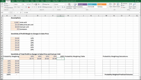 FIGURE 8-11:
Setting up the data table to add
probability weightings.
Now add the data table just as you did in the last section.
- Link B19 to the output cell using the formula =‘Summary’!B8.
- Highlight the entire range B19:F25.
-
Select the What-if Analysis from the Data tab and choose Data Table from the options.
The Data Table dialog box appears.
-
Link the row fi to the input fi for the cost per unit (B5) and the column fi to the input fi for the sales price (B4) and compare your results to those in Figure 8-12.
After you’ve fi the data table, you need to multiply out the probability
weightings into the table so that you can work out how likely each outcome is.
-
In cell H20, add the formula =C$18*$A20.
Don’t forget your mixed cell referencing (see Chapter 6).
-
Copy this formula across the block of data to cell K25 and compare your results to those in Figure 8-12.
The total should add to 100 percent.
-
Add an error check in cell L27 with the formula =1-L26.
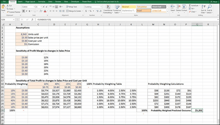
When the data table and the probability weighting table have been built, you can use the results to calculate the probability weighted outcomes.
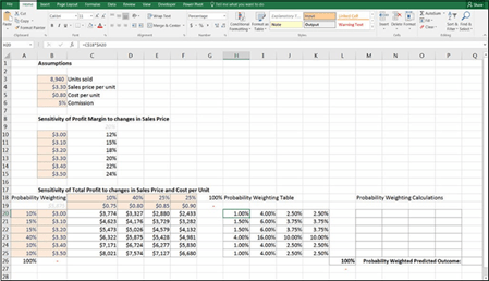 FIGURE 8-12:
Building the probability weighting table.
-
In cell M20, add the formula =H20*C20.
There is no need to add cell referencing for this calculation.
- Copy this formula across the block of data to cell P25 and compare your results to those in Figure 8-13.
-
In cell Q26, add the entire table together with the formula
=SUM(M20:P25), as shown in Figure 8-13.
The calculated result is $5,202, which is the probability weighted predicted outcome of this model. If you’d like to see a completed copy of this model, download File 0804.xlsx from www.dummies.com/go/financialmodeling inexcelfd.
FIGURE 8-13:
Completed probability weighted predicted outcome.
 THE LIMITATIONS OF DATA TABLES
You can see from the examples in this section that data tables are a great way to look at multiple scenarios or sensitivity analyses one at a time. Instead of manually changing the sales price or the cost per unit, you can display at a glance the impact of these changes.
However, data tables have a couple of limitations that make them inappropriate for some scenarios or sensitivity analysis situations:
- The inputs and outputs need to be on the same page.
- You can show only two inputs and one output at a time. This is not a restriction with other forms of scenario analysis.
- Formula auditing (trace precedents and trace dependents) doesn’t work very well in
data tables.
Data tables are extremely useful when you want to see the incremental change of one or two inputs on a single output. Data tables aren’t appropriate if the output of your
fi model is a full set of fi statements, for example. In this situation, a drop-
down scenario would be best.


