Applying Scenarios to Your Financial Model

once (see Chapter 4), adding scenarios to your model is a fairly straightforward process, and including scenarios doesn’t require much work or redesign.
In this chapter, you take a couple of simple models that you’ve already built in previous chapters, and see how simple it is to add scenarios to improve the func- tionality. With a well-built model that has all inputs properly linked through to outputs, changing inputs and watching the outputs change is fairly easy. In fact, you could argue that this is pretty much the whole purpose of building a financial model in the first place!
Scenarios and sensitivity analysis are a great way to reduce risk by seeing all the possible outcomes of the project or venture you’re modeling. What would be the absolute worst that could happen? If everything that can go wrong does go wrong, can you still afford to pay your staff? There are usually interdependent effects and interactions between multiple variables, which may change in the model. That’s
why it’s so important to have links automatically calculating within a model. For example, if units sold increases, then revenue increases, so profitability increases, so cash flow increases, so borrowing decreases, so interest payable decreases, and so on. . . .
Scenarios can also help you make decisions. After you’ve built scenarios into the model, the hypothetical outcomes can be laid out so that the decision makers can see the expected impact of each course of action. How closely these outcomes reflect reality depends, of course, on the accuracy of the model as well as the assumptions that have been used — but you already knew that!
Identifying the Diff between
Types of Analysis
Scenario analysis, sensitivity analysis, and what-if analysis are all very similar to each other. In fact, they’re really only slight variations of the same thing. Here’s a breakdown:
» What-if analysis: What-if analysis is the process of testing to see “what would happen if” you change something in the model.
» Sensitivity analysis: Sensitivity analysis is the process of tweaking one key input or driver in a fi model and seeing how sensitive the model is to the change in that variable.
For example, if you have an income statement with a profi of $1.2 million, you may want to know how that profi is aff by changes in price. If you reduce the per unit price of one of the products from $5.25 to $4.75, the profi may decrease to $975,000, so you can see that the business is quite sensitive to changes in the price for that product. This process of changing a single input in isolation is referred to as performing sensitivity analysis.
» Scenario analysis: Scenario analysis is the process of tweaking a whole series of inputs or drivers in a fi model and seeing what happens with the model.
For example, a worst-case scenario could include not only the price decreasing but interest rates increasing, number of customers decreasing, and unfavor- able exchange rates. Sometimes these inputs aff each other — for exam- ple, a reduction in sales aff profi may also cause sales commission or bonuses to go down, which would also aff profi
Building Drop-Down Scenarios
The most commonly used method of building scenarios (and the one that I most often teach in my training courses) is to use a combination of formulas and drop- down boxes. In the model, you create a table of possible scenarios and their inputs and link the scenario names to an input cell drop-down box. The inputs of the model are linked to the scenario table. If the model has been built properly with all the inputs flowing through to the outputs, then the results of the model will change as the user selects different options from the drop-down box.
Data validation drop-down boxes are used for a number of different purposes in financial modeling, including scenario analysis. For an example of using data validations to reduce errors in a financial model, turn to Chapter 12.
Using data validations to model
profi scenarios
In Chapter 7, you create a simple one-page model to calculate costs based on par- ticular inputs. I recommend that you build the model as described in Chapter 7 first so that you understand how this simple model works before adding the sce- narios to it. Alternatively, you can find a copy of the completed model by down- loading File 0801.xlsx from www.dummies.com/go/financialmodelinginexcelfd. Open it and select the tab labeled 8-1-start.
The way I’ve modeled this, the inputs are lined up in column B. You could perform sensitivity analysis simply by changing one of the inputs — for example, change the customers per call operator in cell B3 from 40 to 45, and you’ll see all the dependent numbers change. This would be a sensitivity analysis, because you’re changing only one variable. Instead, you’re going to change multiple variables at once in this full scenario analysis exercise, so you’ll need to do more than tweak a few numbers manually.
To perform a scenario analysis using data validation drop-down boxes, follow these steps:
-
Take the existing model that you created in Chapter 7 (or downloaded), and cut and paste the descriptions from column C to column F.
You can do this by highlighting cells C6:C8, pressing Ctrl+X, selecting cell F6, and pressing Enter.
The inputs in cells B3 to B8 are the active range that drives the model and will remain so. However, they need to become formulas that change depending on the drop-down box that you’ll create.
-
Copy the range in column B across to columns C, D, and E.
You can do this by highlighting B3:B8, pressing Ctrl+C, selecting cells C3:E3, and pressing Enter. These amounts will be the same for each scenario until we change them.
-
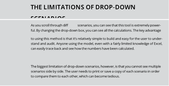
In row 2 enter the titles Best Case, Base Case, and Worst Case, as shown in Figure 8-1.
Note that the formulas still link to the inputs in column B, as we can see by
selecting cell C12 and pressing the F2 shortcut key as shown in fi 8-1.
 FIGURE 8-1:
Setting up the model for scenario analysis.
-
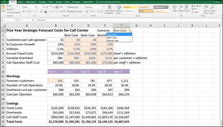
Edit the inputs underneath each scenario.
You can put whatever you think is likely, but in order to match the numbers to those in this example, enter the values as shown in Figure 8-2. Ignore column B for now.
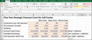 FIGURE 8-2:
Inputs for
scenario analysis.
Now you need to add the drop-down box at the top, which is going to drive your scenarios. It doesn’t really matter where exactly you put the drop-down box, but it should be in a location that’s easy to fi usually at the top of the page.
- In cell E1, enter the title Scenario:.
-
Select cell F1, and change the formatting to input so that the user can see that this cell is editable.
The easiest way to do this is to follow these steps:
- Click one of the cells that are already formatted as an input, such as cell E3.
- Press the Format Painter icon in the Clipboard section on the left-hand side of the Home tab. Your cursor will change to a paintbrush.
- Select cell F1 to paste the formatting.

 Format Painter is normally for single use. After you’ve selected the cell, the paintbrush will disappear from the cursor. If you want the Format Painter to become “sticky” and apply to multiple cells, double-click the icon when you select it from the Home tab.
 - Click one of the cells that are already formatted as an input, such as cell E3.
-
Now, in cell F1, select Data Validation from the Data Tools section of the Data tab.
The Data Validation dialog box appears.
- On the Settings tab, change the Allow drop-down to List, use the mouse to select the range =$C$2:$E$2 (see Figure 8-3), and click OK.
- Click the drop-down box, which now appears next to cell F1, and select one of the scenarios (for example, Base Case).
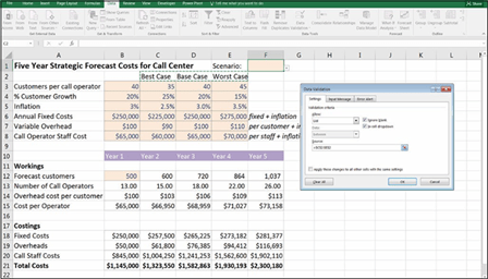 FIGURE 8-3:
Creating the data
validation drop-down scenarios.
Applying formulas to scenarios
The cells in column B are still driving the model, and these need to be replaced by formulas. Before you add the formulas, however, you should change the format- ting of the cells in the range to show that they contain formulas, instead of hard- coded numbers. Follow these steps:
- Select cells B3:B8, and select the Fill Color from the Font group on the Home tab.
-
 Change the Fill Color to a white background.
It’s very important to distinguish between formulas and input cells in a model. You need to make it clear to any user opening the model that the cells in this range contain formulas and should not be overridden.

Now you need to replace the hard-coded values in column B with formulas that will change as the drop-down box changes. You can do this using a number of different functions; an HLOOKUP, a nested IF statement, an IFS, and a SUMIF will all do the trick. Add the formulas by following these steps:
-
Select cell B3, and add a formula that will change the value depending on what is in cell F1.
Here is what the formula will be under the diff options:
• =HLOOKUP($F$1,$C$2:$E$8,2,0)
Note that with this solution, you need to change the row index number from 2 to 3 and so on as you copy the formula down. Instead, you could use a ROW function in the third fi like this: =HLOOKUP($F$1,$C$2:$E$8, ROW(A3)-1,0)
• =IF($F$1=$C$2,C3,IF($F$1=$D$2,D3,E3))
• =IFS($F$1=$C$2,C3,$F$1=$D$2,D3,$F$1=$E$2,E3)
• =SUMIF($C$2:$E$2,$F$1,C3:E3)

 As always, there are several diff options to choose from and the best solution is the one that is the simplest and easiest to understand. Any of these functions will produce exactly the same result, but in my opinion, having to change the row index number in the HLOOKUP is not robust, and adding the ROW may be confusing for a user. The nested IF statement is tricky to build
and follow, and although the new IFS function is designed to make a nested IF function simpler, it’s still rather unwieldy. I fi the SUMIF quite simple to build and follow, and it’s easy to expand if you need to add extra scenarios in the future.
 Note that IFS is a new function that is only available with Offi 365 and Excel 2016 or later installed. If you use this function and someone opens this model in a previous version of Excel, she can view the formula, but she won’t be able to edit it.
-
Copy the formula in cell B3 down the column.

 By using an ordinary copy and paste, you’ll lose all your formatting. It’s important to retain the formatting of the model so that you can see at a glance which inputs are in dollar values, percentages, or customer numbers. Use Paste Formulas to retain the formatting. You can access it by copying the cell onto the clipboard, highlighting the destination range, right-clicking, and selecting the Paste Formulas icon to paste formulas only, and leave the formatting intact (see Figure 8-4).
Now for the fun part! It’s time to test the scenario functionality in the
model.
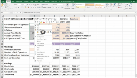 FIGURE 8-4:
Using Paste Formulas to retain formatting.
- Click cell F1, change the drop-down box, and watch the model outputs change as you toggle between the diff scenarios, as shown in Figure 8-5.
FIGURE 8-5:
The completed scenario analysis.