Home » Civil Engineering Projects » Financial Modeling in Excel Budgeting for Capital Expenditure and Depreciation

Civil Engineering Projects

Financial Modeling in Excel Budgeting for Capital Expenditure and Depreciation

learn

April 22, 2023

102 Views 0

SaveSavedRemoved 0

Budgeting for Capital Expenditure and Depreciation

In Chapter 10, I explain the process of purchasing assets and calculating their depreciation. For example, you purchased a coffee machine, as well as fixtures and fittings. These purchases were reflected in your cash flow statement, but you also needed to calculate their depreciation based on their useful life. You used this amount in the Income Statement and showed it on the Balance Sheet in order to show the current value of fixed assets. The way this was calculated was fairly simple.

In this chapter, I explain in more detail how to model depreciation. Here, you take a list of existing and budgeted CapEx items, convert them into a cash flow schedule, calculate the depreciation, and use the depreciated amounts to calculate the written-down value on the Balance Sheet. You also see what happens when an asset is fully depreciated and how to model this.

Getting Started

In this case study, you’re charged with assembling the CapEx component for the coming year’s IT budget. You’ve managed to pull from the fixed assets register a list of assets, the purchase price, and the purchase date. You also have a wish list of items your department wants included in the next budget. You use the informa- tion you have to model the cash flow and the depreciation.

It’s always a good idea to start a modeling project with the end in mind. The outputs that you want to show in this model are the following:

» Output 1: Cash required for asset purchases over the budget period (for the

cash fl    statement)

» Output 2: Depreciation for the budget period (for the income statement)

» Output 3: Written-down value of assets for the budget (for the balance sheet)

You can download the blank template, File 1201.xlsx, at www.dummies.com/go/
financialmodelinginexcelfd. The Calculations tab contains the data you already know and is designed for changes to be made by the user (a colleague or client who is not necessarily expected to understand how the model works) or yourself at a later date. The Assumptions tab contains assumptions you know; anything else you think of during the model-building process can be documented here as well.

The first thing you need to do is enter the time frames. Almost every model has an element of time series data, and it’s important to get this right from the start. You need to decide at what level of time series detail the model should be built. For more information on modeling time frames, see the section in Chapter 3. Most budget models, like this one, will be monthly. Many models are annual, such as the DCF model built in Chapter 11. Some are modeled weekly and many, such as cash flow models, are calculated on a daily basis.

In the following sections, you set up the model template with a variable time series so that the model will be reusable in the future. You also set up the titles, which also calculate dynamically as time goes by.

Making a reusable budget model template

When building the time series for this model, you can easily type in Jan-19, Feb-19, and so on into the Calculations tab, but by doing this, the model can be used only once in its current form. If you want to use it again, the following year, you’d need to update each and every date manually.

A much better idea is to enter the start date as an assumption, using a named range, and each time you use it in the model, refer to the named range. For more information about creating, using, and deleting named ranges, see Chapter 6.

Follow these steps to set up the time series for the budget template:

• Select the Assumptions tab and select cell B2, which contains the budget model start date.
  
• Type Start in the name box in the upper-left corner, as shown in Figure 12-1.
  

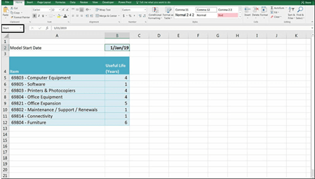FIGURE 12-1:

Creating a named range for the budget model start date.

Now you can use this named range in your formulas as a starting point to model the time series.

• Select the Calculations tab and in cell H2, type =Start.
  

  The value Jan-19 appears. Note that the day of the month does not show because of the way cell H2 has been formatted.
  

• In the Font section on the Home tab, change the font color to white, as shown in Figure 12-2.
  

  In cell I2, you now need to add the rest of the dates. Instead of typing it in manually, you should link it to the start date now in cell H2. There are 31 days in January, so the formula =H2+31 would do the trick but copying it across would make your dates slightly inaccurate and cause problems later on.
  

  Instead, you can use an EDATE function.
  

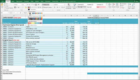FIGURE 12-2:

Changing the font color.

• Select cell I2, and enter the formula =EDATE(H2,1).
  

  By entering the 1 in the second part of the formula, you’re given a date that is exactly one calendar month from the start date (H2). The value in cell I2
  

  is Feb-19.
  

• Copy cell I2 all the way across the row to S2, so that you have all months entered from Jan to Dec.
  

  Just for fun, go back to the Start date assumption on the Assumptions page, and enter the formula =TODAY(). It will show the month and year of today’s date. Go back to the Calculations page, and you’ll see that the budget starts from this month and runs for 12 months into the future. Use the Ctrl+Z shortcut to undo and change the start date back to Jan-19.
  

  While you’re here, you should also add in the dates for the depreciation calculations from column Y onward.
  

• Select cell Y2.
  

  Now, you could simply link this cell back to cell H2, but that would be a case of spaghetti links (see Chapter 14). It will work, but it’s not good modeling practice.
  

• Copy all the cells in the range H2 to S2 across to Y2 to AJ2.
  

  This will link back to the source. Now you’re ready to build the budget.
  

Creating dynamic titles

Before you get into the modeling, take a moment to update the titles in red. It’ll be helpful to show the year in the title, but you don’t want to hard-code the year, because that means the template can’t be reused. Instead, use the YEAR() formula coupled with the ampersand (&) to make a dynamic title:

• Select cell A1 and edit the formula to =”CAPEX BUDGET “&YEAR(Start).
  
• Change the font to black if necessary.
  
• Select cell A11, and enter the formula =”Budgeted Spend “&YEAR(Start).
  

These two formulas in cell A1 and A11 will pull out the year of the start date only, and will automatically change when the start date changes. For another example of using the ampersand in dynamic text, see the example of linked dynamic text in Figure 4-4 (see Chapter 4).

Output 1: Calculating Cash Required for Budgeted Asset Purchases

Now that you’ve set up the layout of the model, you can start to model the num- bers. The Calculations page contains all the information you need to create a cash flow schedule and calculate the depreciation. The top section you’d obtained from the fixed assets register, and the second part is the budget for the coming year.

The first thing you need to do is calculate the total line item amounts in column

E. Follow these steps:

about the prior period for now — just focus on comparing the dates in the time series to the spend date in order to populate the cash fl    schedule.

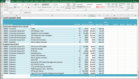FIGURE 12-3:

Calculating total CapEx.

• In cell H4, enter =IF($F4=H$2,$E4,0).
  

  The calculated value in cell H4 is zero because the spend in row 4 occurred in the prior year, not Jan-19.
  

  Be sure to use your mixed cell referencing (using the dollar signs) correctly. For a refresher, see Chapter 6.
  

• Copy this formula all the way across and down the block of data.
  

  By doing this, you’re following good modeling practice by having consistent formulas in blocks of data wherever you can.
  

• Compare your totals to Figure 12-4.
  

  If the referencing has been done correctly, most of the values should be zero, with a few values showing.
  

  You’ll notice that no values are showing for the prior period in column G. You need to add a diff    formula here, which shows the spend value only if the spend occurred prior to the start date of the model. Again, refer to the named range you created earlier because the start date is an arbitrary value that will change.
  

• Select cell G4 and enter =IF(F4<=Start,E4,0). The calculated value in cell G4 is $5,250.
  
• Copy the total in cell E25 across the range G25 to S25.
  
• Compare your totals to Figure 12-4.
  

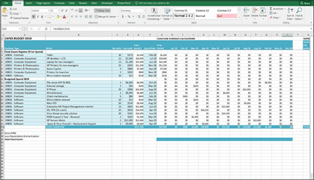FIGURE 12-4:

The completed

cash flow schedule.

Take a moment to understand what this sheet is now telling you. You’ve taken the total spend for each item in column E and spread it out over the full year. The totals of each of the columns G through S should be equal to the total of column

E. If they aren’t, you need to figure out why.

A good financial modeler is always looking for opportunities to include error checks in her financial model. Here’s a good example of where you can include one. For more information about error checks, see Chapter 4.

Follow these steps:

• Select cell E26 and enter the formula =E25-SUM(G25:S25). The calculated value will be zero because the totals are identical.
  
• If you want, use conditional formatting to color the entire cell red if the
  

  error check has been triggered.
  

  If you choose to do this, select Conditional Formatting on the Home tab of the Ribbon, click Highlight Cells Rules, select More Rules, and create a new rule under Format Only Cells That Do Not Contain a Zero. Change the formatting to red fi
  

  Now let’s test the error check to see if it works.
  

• Select cell F12 and change the value to Oct-20 instead of Oct-19.
  

  The error check in cell E26 is triggered because that date is outside the range of the budget schedule and is not being picked up.
  

• Select cell F12 again, and type in 10/15/19 (or 15/10/19, depending on your regional settings) to enter Oct 15, 2019.
  

  Even though the date is within the budget schedule range, the cost in row 12 still isn’t being picked up! This is because the dates in row 2 are actually the fi
  

  of each month (even though it has been formatted to show only the month and the year) so it won’t pick up 15th of the month because the formula is only looking for the 1st. This kind of error is really easy to make, and it’s a good example of how an error check can identify an error that’s been made by a user after the model is complete.
  

Now that you’ve identified this error, you need to correct it and ensure that the same mistake doesn’t happen again going forward. There are a couple of different ways of handling this:

» You can manually change October 15 to October 1. This method is not recommended because, although it’ll correct the error in this instance, it won’t stop any users from making the same mistake again.

» You can insert an extra column to the right of column F, and convert each date that has been entered to the fi    of the month using a formula such as =EOMONTH(F4,-1)+1. This method will work, but you’ll

need to make it clear to the user that any date that is entered will be con- verted to the 1st; otherwise, users will be under the mistaken impression that any date that is entered will have the exact number of days for the deprecia- tion calculations.

» You can stop the user from entering incorrect data in the fi    place.

My preferred solution for this problem is to stop the user from entering an incor- rect value in the first place, using data validations. Follow these steps:

• Select the range F4 to F24 and then select Data Validation from the Data Tools section of the Data tab.
  

  The Data Validation dialog box appears.
  

• On the Settings tab, change the validation criteria to allow a list and use the mouse to select the range =$H$2:$S$2, as shown in Figure 12-5.
  
• Click OK.
  

Data Validations are used for a number of different purposes in financial model- ing. In this instance, they’re used to restrict entry and avoid user error. They’re also widely used in scenario analysis. For an example of how to do this, turn to Chapter 8.

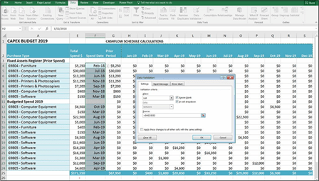FIGURE 12-5:

Restricting errors

with a data validation

drop-down box.

After you’ve added the data validation, you need to document what you’ve done to show users that they can’t simply enter any old data. If they try to enter an invalid date, they’ll get a confusing and frustrating error message unless you explain why.

To prevent user frustration, you can add an input message to the cell so that users know what sort of data they can enter. This will also serve to document this model. For more information on using data validation input messages to document assumptions, turn to Chapter 4.

Follow these steps:

• Select the range F4 to F24 and then select Data Validation from the Data Tools section of the Data tab.
  

  The Data Validation dialog box appears.
  

• Select the Input Message tab, enter some instructions such as those shown in Figure 12-6, and click OK.
  
• Click one of the cells.
  

  The drop-down box, as well as the input message, appears.
  

• Try entering an invalid date, such as October 15, or any gobbledygook.
  

  You get an error message.
  

  You can customize this error message on the third tab of the dialog box if you want.
  

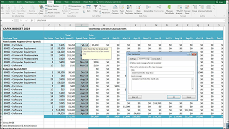FIGURE 12-6:

Using a data validation input message to document the

model.

This means that users cannot enter dates in past periods — which they should not be doing anyway. If you wanted to allow that functionality, you’d need to enter a list of allowable dates elsewhere in the model and link the drop-down boxes to that data instead.

Because this data validation drop-down box is dynamic, the options that appear will change if the dates change. Try this out by changing the start date of the bud- get on the Assumptions from January 19 to January 20. Go back to the drop-down boxes in column F of the Calculations page, and you’ll see that the options avail- able change from dates in 2019 to 2020. When you build the model in this way, making changes in the future is straightforward.

Output 2: Calculating Budgeted Depreciation

Now that the spend has been spread out over the year for the cash flow, you can turn your attention to calculating depreciation. In order to do this, you need a few pieces of information:

» The useful life of the asset

» The written-down date

» The number of months that have elapsed since purchase

Useful life

The useful life can be worked out from the class of the asset, which has already been entered on the Assumptions page. You need to refer to the table using a VLOOKUP function. To review how to use this function, refer to Chapter 7.

Follow these steps to calculate the useful life:

• Select the Assumptions page and select the entire range of asset classes and their useful life.
  
• Highlight the range A4 through B12 and create a named range such as AssetLife, as shown in Figure 12-7.
  

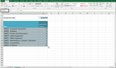FIGURE 12-7:

Creating a named range on the Assumptions

page.

• Return to the Calculations page and, in cell U4, enter the formula
  

  =VLOOKUP(A4,AssetLife,2,0).
  

  The calculated value is 6. This is the number of years the asset will last, but you need to show it in months for your depreciation calculation.
  

• Add *12 to the end of the formula in cell U4 to convert the number of years into months.
  

  The entire formula is now =VLOOKUP(A4,AssetLife,2,0)*12, and the calculated value is 72.
  

Getting units of time mixed up in a situation like this is very easy. Be sure to label carefully. On the Assumptions page, the useful life is shown as Years in the label in cell B4 and on the Assumptions page in cell U2 the label is clearly labeled to show that the time period has been converted to months.

• Copy the formula down the column of data.
  

  An #N/A error appears in cell U11. This happens because of the title in cell A11. You have two options here:
  

  • You can clear the cell so that it’s blank.
    
  • You can add an IFERROR function around the formula and copy it down again. If you choose this option, the formula in cell U4 will be =IFERROR(VL
    

    OOKUP(A4,AssetLife,2,0)*12,0). Then copy it down the range.
    

Written-down date

Now you know when the asset was purchased (or is supposed to be purchased) and you also know how long the asset is expected to last. With these two pieces of infor- mation, you can go ahead and calculate the date at which the asset is expected to be fully depreciated. You can use the EDATE function again just as we did earlier in this chapter to calculate the exact date at which the asset will be fully depreciated.

Follow these steps:

• Select cell V4 and enter the formula =EDATE(F4,U4). The calculated value is Feb-24.
  
• Copy the formula down the range.
  

  Cell V11 returns an incorrect value of Jan-00 again because there is no date value in cell F11 because of the title row. Your options are to:
  

  • Clear the cell so that it’s blank.
    
  • Add an IF statement around the formula that will not calculate the written-down date if no date value has been entered in column F. If you
    

    choose this option, the formula in cell V4 is =IF(F4=0,””,EDATE(F4,U4)). Then copy it down the range.
    

Note that a zero in the first “value if true” field will not work in this instance because a zero result in this formula will simply show as Jan-00. Therefore, a “” is necessary because that will show as a blank value. Be careful, however, when using this technique — a “” value is often treated as text by Excel and can cause some problems in calculations.

The depreciation schedule for the current year

Leave the Months Elapsed Since Purchase and Depn in Prior Period calculations aside for now, and start scheduling out the depreciation from column Y onward. What you need to do here is to show the depreciation only if the schedule date is between the spend date and the written-down date. Or in other words, only if the schedule date is greater than the spend date and less than the written-down date.

This formula is going to be more complex than what we have done so far, as it will contain a nested IF statement. Start by building the first part of the formula; show the depreciation only if the schedule is greater than the spend date. Follow these steps:

• Select cell Y4 and enter the formula =IF(Y$2>$F4,$E4/$U4,0).
  

You can either type the formula directly into the cell or use the Function Arguments dialog box, as shown in Figure 12-8. The calculated value will be $73.

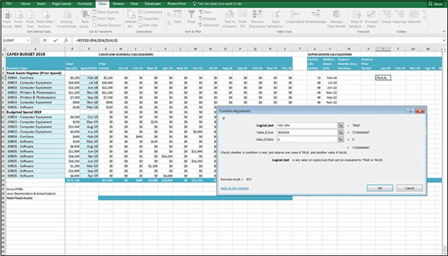FIGURE 12-8:

Using the Function Arguments dialog box to build an IF statement.

Notice that columns B, C, and D are missing from Figure 12-8. This is because Freeze Panes has been added to this document already. Be careful when using sheets with Freeze Panes added — it’s very easy to miss cells in a range when they aren’t showing on the sheet.

This formula takes the cost of the item and divides it by the useful life to calculate the depreciation — but only if the asset has already been purchased. Take special care with the referencing. Be sure to put the dollar signs before the row or the column you want to fi so that we can then copy the exact same formula all the way down and across the block of data.

• Copy the formula across the range Y4:AJ24, and sense-check to make sure that it looks correct.
  

  The depreciation should show only after the spend date has already elapsed on the schedule.
  

  Again, row 11 is causing problems, but you can deal with this later, after you’ve fi    this formula.
  

  Now it’s time to add in the written-down date, which is the second part of the formula, so it should show only if the spend date has elapsed and the written- down date has not elapsed.
  

• Go back to cell Y4 and edit the formula to =IF(AND(Y$2>$F4,Y$2<$V4),
  

  $E4/$U4,0).
  

  The calculated value is still $73.
  

• Ensure that the mixed referencing is correct by inserting the dollar signs in the correct places in the formula, and copy the formula across and down the block of data in the range Y4:AJ24.
  

  Again, you can remove the #N/A errors in row 11 by clearing them or adding the IFERROR function around the formula.
  

• To add the IFERROR function around the formula, in cell Y4 enter =IFERRO R(IF(AND(Y$2>$F4,Y$2<$V4),$E4/$U4,0),0).
  
• Copy this formula across and down the block of data in the range Y4:AJ24.
  
• Select cell Y25 and add a total by pressing Ctrl+=.
  
• Copy this formula across the row to column AJ and compare your totals to those in Figure 12-9.
  

Take a moment to sense-check this depreciation schedule. The first line of defense against error is to check as you go. After you’ve finished the block of data, do a spot check on a random cell such as cell Z14. Select the cells and press F2. This will show you exactly which cells are being used in the formula because they’ll be highlighted, as shown in Figure 12-9. Take a look at cell AA10. Why is it returning a zero value when the cell next to it has a value of $13? This is because the asset has reached the end of its useful life and, therefore, no depreciation should be calculated from March onward.

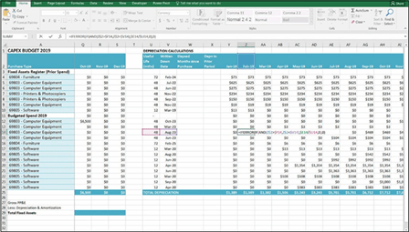FIGURE 12-9:

Calculating depreciation.

Depreciation in prior periods

Now that you’ve calculated the depreciation amounts for the budget year, you can turn your attention to prior years. You need to do this for your Balance Sheet because you need to show the assets at their original purchase price, and then deduct the depreciation to arrive at the current written-down value.

First, you need to work out how many months have elapsed since asset purchase at the beginning of the budget year so that you can figure out how much depreciation to carry forward. You can do this by deducting the budget start date (January 1, 2019) from the asset’s date of purchase (February 1, 2018, for the first asset). The formula =Start-F4 in cell W4 will return the value 334, which is the number of days between the two dates. To convert this number of days to months, you need to divide it by, say, 30 with the formula =(Start-F4)/30. This is probably close enough for our purposes in this model, but it would be more accurate to use a function such as DATEDIF, which calculates the exact number of calendar months between the two dates.

Follow these steps to calculate the amount of time that has elapsed since the asset was purchased:

• Select cell W4 and enter the formula =DATEDIF(F4,Start,”m”).
  

The fi    fi    contains the beginning date, the second fi    contains the ending date of the period, and the third fi    contains the unit of measurement in which to show the resulting value. “d” denotes day, “m” denotes month, and

“y” denotes year.

• Copy this formula down the range W4:W10.
  

  Note that this formula is only relevant for assets purchased in the past, so the bottom half of the schedule can be left blank.
  

  The DATEIF function, although fi    introduced in Excel 2010, is strangely not found in the Function Arguments dialog box. To use the function, you need to type it manually into the cell. It’s rather a mystery why this function did not make it into the Function Arguments dialog box, but it’s a rather handy secret to know!
  

  You can now calculate the depreciation for prior years in column X by dividing the original purchase amount by the useful life to arrive at the monthly depreciation amount. This amount is then multiplied by the number of elapsed months to work out how much depreciation has been incurred in prior years.
  

• Select cell X4 and enter the formula =(G4/U4)*W4.
  
• Copy this formula down the range X4:X10.
  

  Again, note that this formula is only relevant for assets purchased in the past, so the bottom half of the schedule can be left blank.
  

• Copy the sum formula across from cell Y25 to cell X25 to calculate the total for the prior period.
  
• Compare the totals to those in Figure 12-10.
  

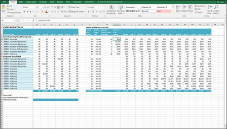FIGURE 12-10:

Depreciation in a prior period.

Output 3: Calculating the Written-Down Value of Assets for the Balance Sheet

For the balance sheet, you need to know how much the asset was originally pur- chased for, and how much has been depreciated to arrive at the written-down value. You already have all the pieces of information that you need to calculate this, and a place to enter it in row 27 of this model. Note that these assets will be called property, plant, and equipment (PP&E) on the balance sheet. For more information on how to incorporate these calculations in a full working financial model, see Chapter 10.

Follow these steps:

• In cell G27, enter =G25+F27 to calculate the total cost of the assets.
  

  This row is a cumulative total that will keep adding more assets as they’re purchased. Note that although there is no value in cell F27, for the sake of formula consistency, you’re still including it so that the formula can be copied across the range consistently.
  

• Copy this formula across the row to column S and compare your figures
  

  to those in Figure 12-11.
  

• In cell G28, enter =-X25+F28.
  

  Again, you include cell F28 for consistency, even though it does not contain a value. The calculated value is –$7,708.
  

• Copy this formula across the row to column S and compare your figures
  

  to those in Figure 12-11.
  

• Add these cells together in cell G29 with the formula =SUM(G27:G28). The calculated value is $60,242
  
• Copy this formula across the row to column S and compare your figures
  

  to those in Figure 12-11.
  

Now that you’ve completed this model, it can be used as a stand-alone model, or each of the completed outputs can be used as inputs for an integrated financial statements model.

You can download the completed version of this model, called File 1202.xlsx, at

www.dummies.com/go/financialmodelinginexcelfd.

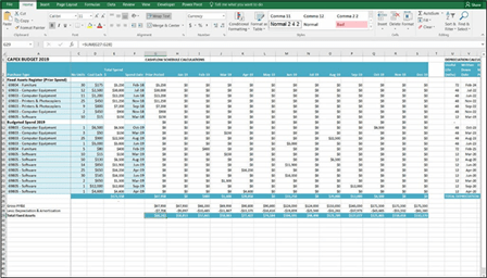
FIGURE 12-11:

The written-down value of assets calculation.