
Exploring New and Useful Workflow Functions
Microsoft Excel 2021 houses some valuable new functions. During this part of the book, you will recap a number of important concepts and investigate some new functions. In the previous book, Learn Microsoft Offi e 2019, we concentrated on the differences between a formula and a function, learned about operators and formula construction, and how to use the correct order of evaluation. We also covered the Function Library and error checking.
This chapter will concentrate on the latest functions involved in learning the syntax and construction of the formula, such as XLOOKUP, LET, and XMATCH, as well as focus on IFS. We will learn to combine formulas, such as IFERROR and VLOOKUP, explore the term ARRAYS, and look at the new dynamic array functions in Excel 2021. There is also a topic included on database functions and a final topic exploring COUNTIFS.
The following list of topics will be covered in this chapter:
- Learning about dynamic arrays
- Investigating new functions
- Exploring database functions
- Using the COUNTIFS statistical function
At the end of the chapter, we will highlight common formula errors and learn how to use named ranges in a formula.
Technical requirements
As you have learned how to insert functions to create a formula and check for errors in the previous edition of our book, we will assume you are equipped with these prerequisite skills. We will now build on these.
The examples used in this chapter are accessible from the following GitHub URL: https://github.com/PacktPublishing/Learn-Microsoft-Office- 2021-Second-Edition.
Learning about dynamic arrays
Let’s first understand the term array and when to use it. An array is simply a collection of data that can be stored in one or multiple rows or columns. Data within these columns
can be numbers or text. In Excel, an array is a formula that performs multiple calculations on one or more items in an array.
Array formulas can return multiple or single results. We can use arrays to eliminate and speed up the number of actions we need to perform in Excel to produce a result. To follow along with the next example, open the workbook named Arrays.xlsx.
For instance, in the example that follows, the usual method you could implement to arrive at a grand total for the cost of each course would be to work out the total amount for each course and then sum the totals to establish the grand total.
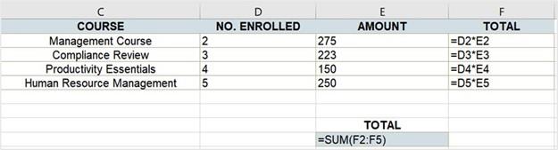
Figure 10.1 – Working out grand totals using the traditional method
This method is great, but we could speed this up by making use of an array either for single or multiple actions, thereby achieving processing in one action and saving an enormous amount of time.
To create an array, we would insert curly brackets around the {formula}. We never type the curly brackets; they are inserted using the Ctrl + Shift + Enter keys.
There are a few pointers to make sure you are aware of when using arrays:
- Always look at the formula bar to see whether a formula is part of an array.
- If you need to edit an array formula, the curly brackets will disappear – you need to insert them again using Ctrl + Shift + Enter at the end of the formula.
- Manually inserted curly brackets will not convert the formula into an array.
Let’s look at how we construct an array formula to eliminate multiple actions (keystrokes).
Constructing an array formula to calculate a total
We will now run through the steps to create an array:
- Using the Arrays.xlsx worksheet, click into cell E9 and then type the following formula: =sum(D2:D5*E2:E5).
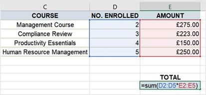
Figure 10.2 – Working out grand totals using an array
- Press the Ctrl + Shift + Enter keys to create the array, after which you will see the total in E9.
- In the formula bar, you will notice the formula has now included curly brackets at the start and end of the formula to enclose it.
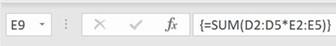
Figure10.3 – The constructed array formula showing curly brackets
- Also take note that when double-clicking in cell E9, the curly brackets are not visible.
Using the array and IF function combined
Let’s explore an array where one range calculates another range to fill in values according to the criteria:
- Using the same workbook as the previous example, we will construct an array formula to display the word HIGH where population growth exceeds 3%. The next screenshot depicts what we would like to achieve as the formula result in cells E16:F19. A change to any of the cells in B16:C19 will automatically update the table in E16:F19.
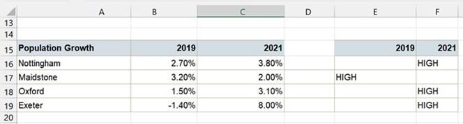
Figure 10.4 – The completed table
-
Select cells E16:F19 and then enter the following formula:
=IF(B16:C19>0.03,”HIGH”,””).
- Press Ctrl + Shift + Enter.
- Amend a growth % value in the first table to see whether the table updates accordingly.
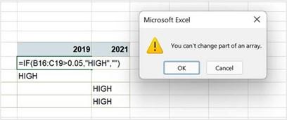
If you make any amends to an array range, it is good practice to highlight the entire range array. For instance, to make amends to the array formula in the previous example, you would select cells E16:F19 to make any changes to the formula. Editing cell E16 and
pressing the Enter key will present an error alert indicating that the cell is part of an array. This is because you have not used the Ctrl + Shift + Enter keys to amend the array.
Figure 10.5 – Error when trying to amend a single cell part of an array


