Financial Modeling in Excel Getting Familiar with the Most Important Functions

April 22, 2023

23 Views 0

SaveSavedRemoved 0

Getting Familiar with the Most Important Functions

You’ve arrived at the meaty part of the chapter. This is where things get interest- ing! In this section, I fill you in on all the functions you’ll rely on most often and give you some examples of how and why to use them.

SUM

As its name implies, the SUM function is used to add a series of numbers. Normally, SUM is used to add a contiguous range of cells, as shown in Figure 7-2, but it can also be used to add cells in a noncontiguous range (in other words, cells that aren’t adjacent to each other).

Figure 7-2 shows an example of adding a column of numbers. To try this out for yourself, select a cell either at the bottom or the far right of a range of cells, and click the Σ AutoSum button on the Home tab or Formulas tab.

FIGURE 7-2:

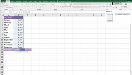
Using the SUM function to add up a column.

When you click the Σ AutoSum button, the SUM function tries to automatically determine the figures that you want to add up — and it usually gets it right. If it hasn’t selected quite the right range you need to sum, you can fix it by doing any of the following:

» Manually edit the range by retyping the references in the Formula Bar.

» Select the correct range of cells with the mouse.

» Drag the plus sign (+) in the corner of the summed range cell to add to the range of cells selected. To do this in the example in Figure 7-2, you would hover the mouse above the upper-right corner of cell B2.

Figure 7-3 shows an example of summing up a specific set of cells in a noncon- tiguous range. Because rows 8 and 15 already contain subtotals, you can’t simply add up the entire column for the full year total — it would include the subtotals as well at the values, so you’d end up with double the number. In the Formula Bar, enter the cell address of each cell that you want added together, so the formula in cell B16 is =SUM(B8,B15). Note that you need to enter a comma to separate each cell (or range of cells) from the others.

Instead of pressing Σ AutoSum, you can use the shortcut Alt+=. Try selecting a cell either at the bottom or the far right of a range of cells, and press Alt+=. The SUM function is inserted, exactly as though you had pressed the Σ AutoSum button. Learning and using shortcuts like this one can save a lot of time when you’re building financial models. See Chapter 6 for more on using shortcuts.

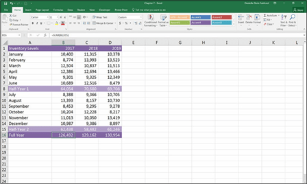FIGURE 7-3:

Using the SUM function to add noncontiguous

cells.

MAX and MIN

The MAX function helps identify the maximum value. The syntax for this function is the same as for the SUM function — you can enter a range of cells, individual cells separated by commas, or a combination of both. The MAX function returns an error if the cells you need to analyze have some text that can’t be converted to numerical values.

For example, if you wanted to determine the maximum sales dollars for a year, you could use the MAX function to do so. In the example shown in Figure 7-4, the MAX function has been used to calculate the highest inventory level for the entire year with the function =MAX(B2:B13). Select cell B14 and you can complete this function in several different ways:

» Type =MAX( and select the range with the mouse or the arrow keys.

» Access the Insert Function dialog box (see “Finding the Function You Need,”

earlier in this chapter), and search for MAX.

» Find the Σ AutoSum button on the Home tab or the Formulas tab (refer to Figure 7-2) and instead of clicking it, select Max from the drop-down box next to the button.

FIGURE 7-4:

Using the MAX function to calculate the maximum value.

The MIN function is the opposite of the MAX function: It calculates the lowest value in the column. The MIN function can also use any combination of ranged series and individual cells. The restrictions on what you enter and the results you get are similar to the MAX function. For example, if you wanted to determine the minimum inventory level for a year, you could use the MIN function, as shown in Figure 7-5 with the function =MIN(B2:B13).

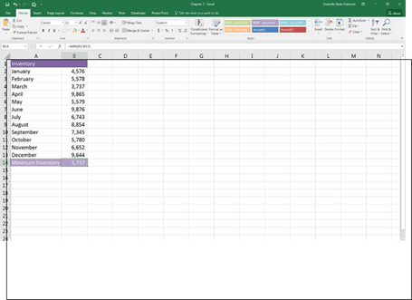
FIGURE 7-5:

Using the MIN function to calculate the minimum value.

Now that you’ve determined both the minimum and maximum values, you can use these formulas to calculate the spread, or variance, of the inventory levels between minimum and maximum values. Maybe your investors want to know how volatile your stock levels are. This calculation will give you some idea of the volatility of inventory.

For a practical example of how to use the MAX and MIN functions together, follow these steps:

Download File 0701.xlsx at www.dummies.com/go/financialmodeling inexcelfd, open it, and select the tab labeled 7-6, or open a new Excel fi and enter and format the data as shown in Figure 7-6.

FIGURE 7-6:

Three years of

inventory levels.

In cell B16, enter the function =MAX(B2:B13) to calculate the maximum

inventory level for the fi year.
Copy that function across the row — in cells C16 and D16 — so that it

calculates for all three years.

Because you want the cell referencing to change as you copy it across, no

anchoring or dollar signs are required on the cell references.
In cell B17, enter the function =MIN(B2:B13) to calculate the minimum

inventory level for the fi year.
Copy that function across the row — in cells C17 and D17 — so that it

calculates for all three years.

In cell B18, enter the formula =B16-B17 to calculate the spread by deducting the minimum value from the maximum value.
Enter the titles “Maximum,” “Minimum,” and “Spread” in cells A16:A18, as shown in Figure 7-7.
Copy that formula across the row — in cells C18 and D18 — so that it

calculates for all three years.

The completed model is shown in Figure 7-7. Note that the second year has the widest range, with a spread of 5,836.

FIGURE 7-7:

Inventory Spread

over three years.

This calculation could also have been done in a single row, using the formula

=MAX(B2:B13)-MIN(B2:B13), but using this approach to building simple formulas first in separate cells makes your model easy to follow and it’s sometimes neces- sary before attempting to build complex formulas. You can always put them together later, after you figure out what intermediary calculations you need.

AVERAGE

What if you have several hundred cells in a single spreadsheet column, each with a numerical value, and you want to find the average, or mean, value? Using ordi- nary formulas, you would have to sum all the numbers up, count the number of rows, and then divide the sum by the number of rows. Fortunately, Excel has an AVERAGE function, which makes this calculation a lot easier.

In the example shown in Figure 7-8, I quickly and easily calculated the average value of 7,019 with the AVERAGE function.

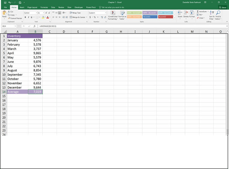
FIGURE 7-8:

Using the AVERAGE

function to calculate the average value.

The AVERAGE function only uses the cells with values. Make sure that this is what you intend with your calculation. In most situations, there isn’t a lot of difference between a blank cell and a cell containing a zero value — and most functions treat a blank cell as though it contains a zero. When using the AVERAGE function, how- ever, this is not the case. The AVERAGE function counts the cells with value zero, but it ignores empty cells and doesn’t include them in the calculation. If you want those cells to be counted, you need to enter a value of zero in the cells.

In the example shown in Figure 7-9, I don’t have any data yet for December, so cell B13 has been deliberately left blank. Although cell B13 has been included in the AVERAGE function’s range, the function ignores it, and calculates the correct average for January to November as 6,780.

In the example shown in Figure 7-10, the user has entered a zero value in cell B13 instead of leaving it blank. The AVERAGE function includes this zero value when calculating the average, giving the value of 6,215.

COUNT and COUNTA

The COUNT function, as the name suggests, counts. Although this sounds pretty straightforward, it’s actually not as simple as it seems and, for this reason, the COUNT function is not as commonly used as the very closely related COUNTA function.

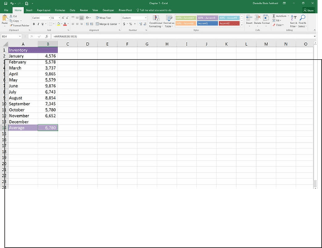
FIGURE 7-9:

The AVERAGE

function ignores

blank cells.

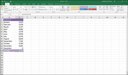
FIGURE 7-10:

The AVERAGE

function includes zero values in its

calculation.

The COUNT function only counts the number of cells that contain numerical val- ues in a range. It will completely ignore blank cells and any cells within the range that don’t contain numerical values, such as text. For this reason, the COUNT function is used only if you specifically want to count the numbers only.

In the example shown in Figure 7-11, I’m in the preliminary stages of planning for a wedding, and I need to calculate a couple different numbers from the data. I need to know the number of guests to be invited in order to figure out the maxi- mum capacity for the venue. I also need to know the number of invitations to

send, so I can order them from the printers. I’m not sure yet how many people are in the Fleming family, so I’ve inserted a question mark for now. The number of guests can be easily calculated using the SUM function; if I update the numbers in the future, the sum will automatically change without a problem. I can use the COUNT function to calculate the number of invitations, with the formula

=COUNT(B3:B13), but it will entirely ignore the cell containing the question mark and lead me to only order 10 invitations instead of 11.

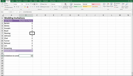
FIGURE 7-11:

The COUNT

function ignores cells without numerical values.

The COUNTA function would be a much better solution to the problem shown in Figure 7-11. In fact, COUNTA is often used instead of COUNT. This is because the COUNTA function will count all cells containing data, not just numerical values, including error values and empty text (“”), but it will still ignore cells that are completely empty.

In the wedding-planning example, I could use the formula =COUNTA(B3:B13) instead, and this will give the correct result. Remember: The COUNTA function ignores blank cells, so if you were to remove the question mark from cell B7 and leave it blank, the answer would be incorrect again. A better solution would be to count the number of names in column A, using the formula =COUNTA(A3:A13), as shown in Figure 7-12.

Calculating a full-year projection using COUNT functions

Let’s try calculating a full-year projection using the COUNT and COUNTA func- tions. For example, say you have only ten months of data, and you want to do a full-year projection for your monthly budget meeting. As shown in Figure 7-13,

you can calculate how many months’ worth of data you have by using the formula

=COUNT(B2:B13), which will give you the correct number of elapsed months (10).

To insert the function, you can either type out the formula in cell B15 (as shown in Figure 7-13), or select Count Numbers from the drop-down list next to the Σ AutoSum button on the Home tab or the Formulas tab.

Note that the COUNTA function would work just as well in this case, but you particularly want to count only numbers, so you should stick with the COUNT function this time.

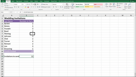FIGURE 7-12:

The COUNTA

function only

ignores

empty cells.

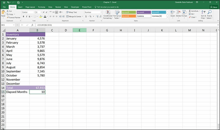
FIGURE 7-13:

Using the COUNT function to count the number of values in a range.

Try adding a number in for November, and notice that the elapsed months changes to 11. This is exactly what you want to happen because it will automatically update whenever you add new data.

In cell B16, calculate the average monthly amount of inventory for the months that have already elapsed. You can do this using the formula =B14/B15. Then you can convert this number to an annual amount by multiplying it by 12. So, the entire formula is =B14/B15*12, which yields the result of 81,520, as shown in Figure 7-14.

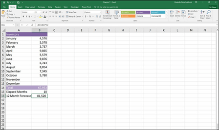FIGURE 7-14:

A completed 12-month forecast.

You can achieve exactly the same result using the formula =AVERAGE(B2:B13)*12. Which function you choose to use in your model is up to you, but the AVERAGE function does not require you to calculate the elapsed number of months as shown in row 15 in Figure 7-14. My personal preference is to see the number of months shown on the page so I can make sure the formula is working correctly.

Calculating headcount costs with the COUNT function

Let’s take a look at another example where the COUNT function can be useful. I often use the COUNT function to calculate headcount in a budget as it’s entered. For a practical example of how to use the COUNT function as part of a financial model, follow these steps:

Download File 0701.xlsx from www.dummies.com/go/financialmodeling inexcelfd, open it, and select the tab labeled 7-15 or enter and format the data as shown in Figure 7-15.

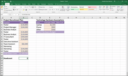FIGURE 7-15:

Using a COUNT function to calculate headcount.

In cell B17, enter the formula =COUNT(B3:B14) to count the number of

staff in the budget.

You get the result of 9.

Again, the COUNTA function would’ve worked in this situation, but I specifically wanted to add up only the number of staff for which I have a budget.

Try entering TBD in one of the blank cells in the range. What happens? The COUNT function doesn’t change its value because it only counts cells with numerical values. Try using the COUNTA function instead (with TBD still in place in one of the formerly blank cells). The result changes from 9 to 10, which may or may not be what you want to happen.

After you’ve calculated the headcount, you can incorporate this information into your technology budget. Each of the costs in the budget is a variable cost driven by headcount. Follow these steps:

In cell F3, enter the formula =E3*B17.

This formula automatically calculates the total cost of all laptops based on the

headcount numbers.

Because you want to copy this formula down, you need to anchor the cell

reference to the headcount.
Change the formula to =E3*$B$17 by using the F4 shortcut key or typing in the dollar signs manually.
Copy the formula down the range, and add a total at the bottom, as shown in Figure 7-16.

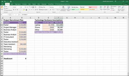FIGURE 7-16:

The completed

budget.

ROUND, ROUNDUP, and ROUNDDOWN

Several Excel functions round off numbers. The ones that are the most useful for financial modelers are ROUND, ROUNDUP, and ROWNDOWN. The ROUND func- tion rounds to the nearest specified value — whether it’s up or down. The ROUNDUP function rounds up to the nearest specified value. And — you guessed it — the ROUNDDOWN function rounds down to the nearest specified value.

To understand how this particular function works, try it out for yourself by fol-

lowing these steps:

Open a new fi in Excel.
In cell A1, enter the number 45215754.575.
On the Home tab, in the Numbers section, click the comma button once to format the cell.

The formatting changes so the number now looks like this: 45,215,754.58. Note that the number remains the same; the third decimal place is still there but it’s just not showing due to the way the cell is formatted.
Select the blank cell A2, enter the formula =ROUND(A1,1).

The 1 in the last part of the formula means that you only want one decimal place. The decimal places are reduced to only one so that cell A2 contains the value 45,215,754.60. Note that the number really does only contain one decimal place; the extra decimal places are not being suppressed by formatting as they are in cell A1.

Now select the blank cell A3, and enter the formula =ROUND(A1,0) to remove all decimal places completely.

The result is 45,215,755.00. Now the cell value contains no decimal places at all.
In the blank cell A4, enter the formula =ROUND(A1,-1) to round the number to the nearest ten.

The result is 45,215,750.00
In cell A5, enter the formula =ROUND(A1,-3) to round the number to the nearest thousand.

The result is 45,216,000.00.
In cell A6, enter the formula =ROUND(A1,-6) to round to the nearest million.

The result is 45,000,000.00, as shown in Figure 7-17.

FIGURE 7-17:

Using the ROUND

function.

For a practical example of how the ROUNDUP and ROUNDDOWN functions are used in a financial model, see the Corkscrew Cash Flow case study in Chapter 11.

Now let’s look at an example of how to use the ROUNDUP function as part of a financial model. Let’s say you’re building a five-year plan for a call center. Each call operator can handle 40 customers. In the first year, you have 500 customers,

and you expect that to increase by 20 percent per year. You have fixed costs of

$250,000. The variable overheads are $100 per customer. Each call operator costs

$65,000 per year. And all costs increase by inflation of 3 percent. How many call operators will you need each year? (Hint: Don’t forget to round up!)

This exercise demonstrates the difference between fixed, variable, and stepped costs, which are important concepts in management accounting and budget mod- eling. As shown in Figure 7-18, fixed costs do not change as the number of units produced increases. Variable costs change directly in line with the number of units produced, and are also very simple to model. Stepped costs, however, do not increase in a linear fashion; instead, they increase in increments or “steps,” and these can be modeled using the ROUNDUP function.

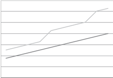
FIGURE 7-18:

Fixed, variable, and stepped

costs.

This exercise also demonstrates a common escalation technique for increasing amounts by a growth rate, or inflation amount. You’ll often need to be able to include escalation in your models for the purpose of forecasting, as you do in this exercise. In this exercise, you need to increase your number of customers by 20 percent each year. The number of customers in the first year is 500. When you add the 20 percent growth to this number, it becomes 600. Then you calculate the cus- tomer number in the third year based on this number (600) not the first year (500). This effect, whereby the growth increases exponentially, is called compounding.

To calculate growth, use the following formula:

Base Amount × (1 + Growth)

You’re adding 1 (effectively 100 percent) to the growth rate (which is 20 percent)

because you want the capital sum returned along with the accrued interest.

Multiplying an amount by (1 + Growth) is a very common calculation in financial

modeling.

Okay, finally, to answer the question posed earlier — “How many call operators will you need each year?” — follow these steps:

Download File 0701.xlsx from www.dummies.com/go/financialmodeling inexcelfd, open it, and select the tab labeled 7-19 or enter and format the data as shown in Figure 7-19.

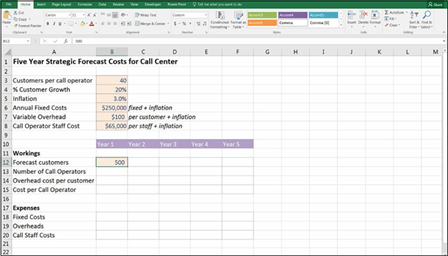FIGURE 7-19:

Calculating number of call

operators required with ROUNDUP.

In cell C12, enter the formula =B12*(1+$B$4) to calculate the number of customers expected in Year 2.

Don’t forget to use the F4 shortcut to anchor the cell reference.

Copy this formula all the way across the row.

The calculated result in Year 5 is 1,037.
In cell B13, you need to work out how many call operators you need each year, so divide the number of customers by the customers per operator with the formula =B12/$B$3.

Don’t forget to use the F4 shortcut to anchor the cell reference.

The calculated result is 12.50.

Huh? That doesn’t make sense. You can’t employ a fraction of a person! You need to round up to the nearest whole person with the formula by wrapping a ROUNDUP function around the existing formula.

In cell B13, change the formula to =ROUNDUP(B12/$B$3,0).
Copy that formula all the way across the row.

The calculated result in Year 5 is 26. Compare your results to Figure 7-20.

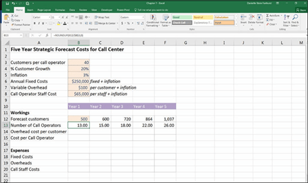FIGURE 7-20:

Calculating number of call

operators required with ROUNDUP.

You’ve now calculated the number of staff required. You can use this information later on in row 20 to work out their costs. For now, let’s continue working down the page.

In row 14, you need to calculate the overhead amounts for each year. There are two parts to this calculation: First, you need to apply inflation, and second, you need to multiply it by the number of customers. You could do the entire calculation in a single row, but the formula would be difficult to follow.

When it comes to formula layout in a financial model, simple is best! It’s far better to lay out the calculation step by step instead of trying to do the whole thing in one row.

Follow these steps to work out how much the staff will cost each year:

In cell B14, enter =B7 to link this to the overhead assumption.
In cell C14, enter the formula =B14*(1+$B$5) to add infl

This technique is exactly the same as the one you used when increasing the number of customers, but you’re picking up the infl assumption instead of the growth assumption.

Don’t forget to use the F4 shortcut to anchor the cell reference.

Copy the formula all the way across the row.

The calculated result in Year 5 is 113.

Note that you have different formulas in cells B14 and C14. Ordinarily, you should try to have consistent formulas wherever possible, to reduce the number of for- mulas in the model, but in this case, it’s just not practical.

In row 15, you need to calculate the staff costs per operator for each year. This works in exactly the same way as the overhead costs. You’ll increase the per- operator costs by inflation each year and multiply it by the number of operators later on. Follow these steps:

In cell B15, enter =B8 to link this cell to the cost per operator.
In cell C15, enter =B15*(1+$B$5) to add infl to this number.

Don’t forget to use the F4 shortcut to anchor the cell reference.

Copy the formula all the way across the row.

The calculated result in Year 5 is $73,158.

You’ve fi the workings block, so you can start to calculate the costs below in row 18.
In cell B18, enter =B6 to link this cell to the fi cost assumption with

the formula.
In cell C18, enter the formula =B18*(1+$B$5) to add infl to this

number.

Copy the formula all the way across the row.

The calculated result in Year 5 is $281,377.
In cell B19, enter the formula =B14*B12 to calculate the total overhead costs by multiplying the overhead cost per customer per year by the number of customers in that year.

No need to lock the cell referencing, because you want this to copy across the row.

Copy the formula all the way across the row.

The calculated result in Year 5 is $116,693.
In cell B20, enter the formula =B15*B13 to calculate the total call staff

costs by multiplying the cost per operator by the number of operators.
Copy the formula all the way across the row.

The calculated result in Year 5 is $1,902,110.
In cell B21, enter the formula =SUM(B18:B20) to sum the total costs.

Another option is to select cell B21 and use the shortcut Alt+=.
Copy the formula all the way across the row.

The calculated result in Year 5 is $2,300,180. Compare your results to Figure 7-21.

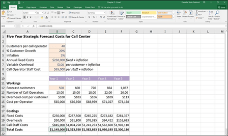FIGURE 7-21:

The completed

five-year strategic

forecast.

The IF function is very commonly used in financial models because it allows you to test certain conditions in your model and change outcomes or results depend- ing on what the user inserts into the model. It’s especially useful when building scenarios, because you can build the model so that the user can turn certain con- ditions on and off.

Type =IF and then use the Ctrl+A shortcut. The IF Function Arguments dialog box

appears. There are three fields you need to fill in:

» The logical statement that is evaluated: For example, is the weather sunny

today? The answer to this will either be true or false.

» The result if the statement is true: In this case, it might be “Go to the

beach.”

» The result if the statement is false: In this case, it might be “Stay home.”

The syntax looks like this:

=IF(statement being tested, value if true, value if false),

So, for this example, in plain language, the syntax looks like this:

=IF(the weather is sunny,go to the beach,stay home),

Written in an Excel formula, if the weather has been put into cell A1, the formula

would look like this (see Figure 7-22):

=IF(A1=”Sunny”,”go to the beach”,”stay home”)

When using text within a formula, as you’re doing in this example, you must put quotation marks (“”) around any text. However, if you use the IF Function Argu- ments dialog box, as shown in Figure 7-22, there is no need to put the quotation marks in manually — the dialog box will do it for you.

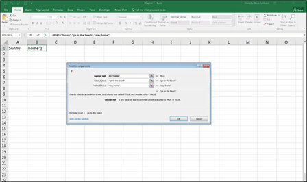
FIGURE 7-22:

Inserting an IF function using the Function Arguments dialog box.

The IF function can be used to automatically calculate whether a set of numbers meets certain conditions. For example, you can create a variance alert when com- paring actual costs to budget — if the variance is greater than 10 percent, you want the formula to automatically alert us. For a practical example of how to use the IF function as part of a financial model, follow these steps:

Download File 0701.xlsx from www.dummies.com/go/financialmodeling inexcelfd
and select the tab labeled 7-23-blank or enter and format the data in columns A through D, as shown in Figure 7-23.
- In cell E3, enter the formula =D3-C3 to calculate the variance.
  
  When preparing an actual versus budget report, you should always show the variance as a positive if it’s “better” than budget or a negative if it’s “worse” than budget. This report shows expenses, so an actual amount higher than budget is a bad thing and should be shown as a negative value. For an expense report, the variance calculation is budget minus actual; for a revenue report, the variance calculation is actual minus budget.
  
  If you’re showing an income or profi and loss statement with revenue at the top part of the report and expenses at the bottom, the formula can’t be exactly the same all the way down the page. Although the consistency of formulas is an important part of fi modeling best practice, it’s not always practical!
- Copy this formula down the column.
  
  When copying down a column, you can select the cell you want to copy, hover the mouse over the lower-left corner until the cross-hairs appear, and double- click. The formula is copied all the way down to the bottom.
- Select cell E13 and use the shortcut Alt+=, and then press enter to sum the column.
  
  The calculated value is $1,555.
- In cell F3, enter the formula =E3/D3 to calculate the variance percentage.
- Copy this formula down the column.
  
  You will notice an error value in row 11. This is because there was no budget for Other IT Costs and the formula can’t divide by zero, so it shows an error value.
- Select cell F3 and suppress this error by editing the formula to
  
  =IFERROR(E3/D3,0).
  
  Any formula errors will show a zero value instead of the error.
- Copy this formula down the column.
  
  Go back to the fi cell (E13) to make the change and then copy it down, instead of making the change only where the error shows (E11). This way, if the numbers change in the future, the errors will always be suppressed.

Ensure that the variance formula also copies all the way down to cell F13 and edit the formatting if necessary.

Now that you’ve set up the actual versus budget report, you can add an IF function to alert you when the variance is too high. First, you need to deter- mine what you mean by “too high.”
In cell G1, enter the value –10%.

You’ll link to this cell because this is the maximum variance to budget you can

tolerate.

Don’t forget to press F4 after referring to G1 to lock the cell reference so that you can copy it down.
In cell G3, type =IF( and press Ctrl+A.

The Function Arguments dialog box appears.
Enter the formula =IF(F3<$G$1,”Over budget”,0), as shown in Figure 7-23.

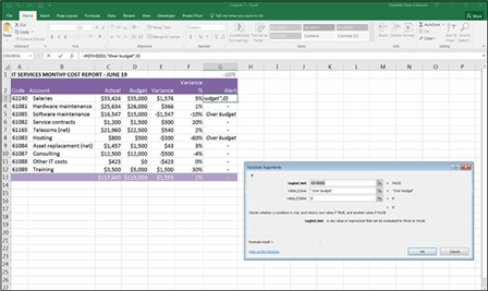FIGURE 7-23:

Building a variance alert

formula.

Ensure that the variance formula also copies all the way down to cell G13 and edit the formatting if necessary.

Your actual versus budget variance report is complete!

The zero values in the G column appear as a dash because of the way the cells have been formatted. This was done using the Comma Style in the Numbers section on the Home tab in the Ribbon. It looks much neater than showing a zero.

COUNTIF and SUMIF

COUNTIF and SUMIF are very handy functions to know for modeling. They add or count ranges of data, and are among some of my favorite, most frequently used functions.

Tallying sales with COUNTIF

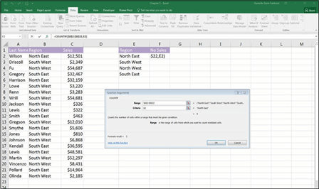
COUNTIF is used to count the number of cells that match specified criteria. For example, you have a list of sales made by salesperson by region, as shown in Figure 7-24. You’d like to know how many sales were made in each region. To solve this problem, follow these steps:

Download File 0701.xlsx from www.dummies.com/go/financialmodeling inexcelfd, open it, and select the tab labeled 7-24.
Copy column B in its entirety to column E, as shown in Figure 7-24.
Leave column E selected, and on the Data tab, in the Data Tools section, click the Remove Duplicates button.

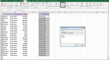FIGURE 7-24:

The Remove Duplicates dialog box.

Click OK.

A message box displays how many duplicate values are to be removed.
Click OK.

The duplicate values are removed, leaving you with a unique list of regions, as

shown in Figure 7-25.

FIGURE 7-25:

The COUNTIF

Function Arguments dialog box.

In cell F1, type No. Sales and format if necessary.
In cell F2, type =COUNTIF( and press Ctrl+A.

The Function Arguments dialog box appears. The Range fi shows the range containing the original data.
Put your cursor in the Range fi and then highlight the cells B2:B22;

press the F4 shortcut key to lock the cell references.
Tab to the Criteria fi and select the fi cell in the table you’re

building (cell E2 as shown in Figure 7-25).

Note that you don’t need to lock this reference because you want the cell

reference to change as you copy it down the column.
Click OK.

The resulting formula will be =COUNTIF($B$2:$B$22,E2) with the calculated

value of 5.
Copy the formula down the column.
Click cell F6, use the shortcut Alt+=, and press Enter to add the sum total.

The calculated value is 21.
Format as necessary.
In cell F7, enter the formula =COUNTA(B2:B22)-F6 to make sure the totals are the same.

Format the zero to a dash by clicking the comma button from the Number section of the Home tab.
Check your numbers against Figure 7-26.

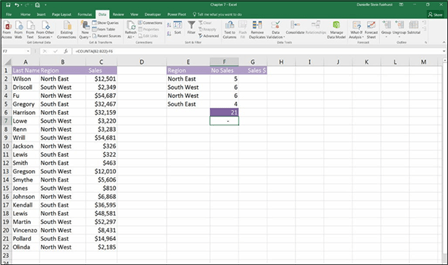FIGURE 7-26:

The completed number of sales

table with

error check.

Reporting sales with SUMIF

SUMIF is similar to COUNTIF, but it sums rather than counts the values of cells in a range that meet given criteria. Following on from the last example, let’s say you want to know how much (in terms of dollar value) in sales were made in each region. To solve this problem, follow these steps:

In cell F1, type “No. Sales” and format if necessary.

In cell F2, type =SUMIF( and press Ctrl+A.

The Function Arguments dialog box appears.
In the Range fi enter the items you’re adding together (B2:B22), and

then press F4.
In the Criteria fi enter the criteria you’re looking for in that range (E2).

You don’t press the F4 key here, because you want to copy it down the column.
In the Sum_range fi enter the numbers you want to sum together

(C2:C22), and then press F4.

Figure 7-27 shows what this should look like.

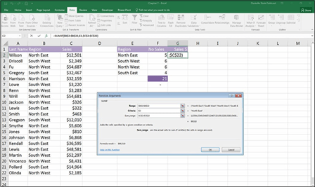FIGURE 7-27:

The SUMIF

Function Arguments dialog box.

Click OK.

The resulting formula will be =SUMIF($B$2:$B$22,E2,$C$2:$C$22) with the

calculated value of $99,310.
Copy the formula down the column.
Click cell G6, use the shortcut Alt+=, and press Enter to add the sum total.

The calculated value is $384,805.
Format as necessary.
In cell G7, enter the formula =SUM(C2:C22)-G6 to make sure the totals are the same.
Format the zero to a dash by clicking the comma button in the Number section of the Home tab.
Check your numbers against Figure 7-28.