
Building the Balance Sheet
The accounting equation as shown on the balance sheet is perhaps the single most important concept to understand in terms of financial statements modeling:
Assets = Liabilities + Shareholders’ Equity
Let’s take a look at each of these components:
» Assets: All property owned by the company. This includes cash in the bank, factories, materials, and even money you’re owed. You can think of assets as the resources that are used to generate revenue.
Assets are split into two categories:
-
Current assets: Current assets can be easily converted into liquid assets or cash. This includes assets such as stocks and shares, account receivables
(money that is owed to the company), and stock that will sell soon for cash.
-
Fixed assets: Fixed assets are still property owned by the company, but they may take longer to convert into liquid assets. This includes large
capital items such as factories or equipment, as well as nonphysical assets such as intellectual property or goodwill.
» Liabilities: All debts owed. Similarly, current liabilities are short-term debt that needs to be paid back within a year, such as accounts payable (money you owe to suppliers), credit card debt, or overdrafts. Long-term liabilities are
more formal borrowings such as bank loans.
» Shareholders’ equity: What the owner has after all the debt has been repaid. If the company were sold, theoretically, this is what the shareholders would have.
The balance sheet shows the financial position of a company at any given moment. Just as with the income statement, the elements of a balance sheet need to be arranged in a specific order:
ASSETS
Current Assets
Fixed Assets
LIABILITIES
Current Liabilities Long-Term Liabilities
EQUITY
Common Stock Additional Paid in Capital Retained Earnings
TOTAL EQUITY
TOTAL LIABILITIES AND EQUITY
Now that you’ve projected your income and cash flow, you need to complete your balance sheet and connect all three financial statements.
Your cafe’s beginning balance sheet at Year 0 will be tied to your sources and uses of funds. Your uses of funds will be your starting assets, and your sources of funds will represent your liabilities and equity. Breaking down the concepts, your uses of funds are assets that you’re purchasing in order to operate the business. Your sources of funds are how you fund the purchases of said assets — money can be raised through liabilities that you owe, such as a bank loan, or it can be equity invested by an owner (in this case, you!).
Start with the current assets (which for your business consists of your cash) and inventory. Follow these steps:
-
On the Balance Sheet worksheet, select cell B5 and enter the formula =’IS
Cash Flow’!B42.
This formula links cell B5 to the closing cash amount you calculated in the last section on the cash fl statement. This represents the starting cash of $5,000 your business has on hand.
-
Select cell B6 and enter the formula =K10.
This formula links cell B6 to the working inventory on the uses of funds you entered earlier on the same worksheet. This represents your starting inventory amount of $5,000.
- Leave accounts receivable in cell B7 blank, and sum the current assets in cell B8 with the formula =SUM(B5:B7); copy the formula across to the second year.
-
Select cell B11 and add cells K11 and K12 on the same worksheet with the formula =K11+K12.
The calculated value is $45,000. This represents your starting PP&E.
- Leave depreciation in cell B12 blank for now and sum the fi assets net of depreciation with the formula =SUM(B11:B12); copy it across to the second year.
-
Sum the current and fi assets in cell B15 with the formula =B13+B8; copy it across to the second year.
This gives you the calculated total asset value of $55,000.
- Leave row 20 blank because you don’t have any current liabilities at this point.
-
Select cell B23 and enter =K3.
This formula links cell B23 to the bank loan amount of $30,000 you entered earlier into the sources of funds section on the same worksheet. This repre- sents the amount you have borrowed from, and owe to, the bank.
-
Sum total long-term liabilities in cell B24 with the formula =SUM(B23) and copy it across to the second year.
It may seem strange to only sum one number, but it’s important to do so for consistency. If at a later date you add other rows for long-term liabilities, they’ll also be included in this total.
-
Select cell B27 and enter the formula =K4.
This formula links cell B27 to the $25,000 equity amount raised that you entered earlier in the sources of funds section on the same worksheet. This represents the amount you’ve invested and your equity in the business.
-
Row 28 relates to retained earnings, which will come from the profi
shown on the income statement.
This is not relevant for Year 0 because you haven’t yet begun operations.
-
Sum total the liabilities and equity in cell B31 with the formula =B29+B24, and copy it across to the second year.
You know that total assets must be equal to liabilities and equity in order for the balance sheet to balance, so this is a perfect opportunity to include an error check.
-
Add an error check in cell B32 with the formula =B31-B15 and copy it across to the second year.
Now that you’ve completed the balance sheet for the pre-open year, you need to link your balance sheet to the income and cash fl statements to deter- mine what the balance sheet will look like after the fi year of operations.
The cafe’s cash at bank will change by the amount of cash fl from your cash fl statement. You’ve already calculated this on a monthly basis, and you have a closing cash fi at the end of December of Year 1.
- Go back to the top of your balance sheet, select cell C5, and link it to the closing cash balance of $19,624 on the IS Cash Flow worksheet with the formula =’IS Cash Flow’!N42.
-
In cell C11, enter the formula =-SUM(‘IS Cash Flow’!C35:N35).
This formula calculates the total amount of fi assets on the books at the end of the second year. If you’ve purchased additional assets during the year, it will show on the cash fl statement, so you need to link that through with the formula. Note that any CapEx purchases on the cash fl statement are
shown as negative values so you need to add a minus sign to the beginning of the sum to show it as a positive value. The total will be zero at this point, but that may change in future iterations of these fi statements.
You also need to add the existing fi asset amount of $45,000 carried over from the previous year.
-
Add this amount to the beginning of the formula you already have in C11 so that it looks like this: =B11-SUM(‘IS Cash Flow’!C35:N35).

 Note that fi assets need to be shown at their original cost (regardless of whether they’ve increased or decreased in value since purchase) and then the accumulated depreciation is shown on a separate line to give us the total written-down value of the asset at that point in time. A long-term asset like the ones shown here will be depreciated until it’s worth nothing on the balance sheet at the end of its useful life.
Because the fi assets’ value is depreciated, you need to pick up the D&A amount already calculated on the income statement.
-
Select cell C12 and enter the formula =-‘IS Cash Flow’!O13.
You need to enter the minus sign because D&A subtracts from gross PP&E.
-
Check your totals.
The total amount of D&A expensed throughout Year 1 is $6,833, total fi assets is $38,167, and total assets is $62,791.
Moving on to liabilities, in cell C23 you need to take into consideration any paying down of debt that may have occurred during the year. If there is any, it would show up in the cash fl on row 40.
-
Although there isn’t any at the moment, you should still link this row through to the balance sheet with the formula =SUM(‘IS Cash Flow’!C40:N40).
The calculated value is zero.
- You then need to add the bank loan carried over from the previous year, so adjust the formula in cell C23 to =B23+SUM(‘IS Cash Flow’!C40:N40).
The calculated value is $30,000.
-
For owners’ funds in cell C27, simply carry this over to the next year with the formula =B27.
Finally, your retained earnings represent the amount of economic profi or net income, your business has earned that has been retained in the company. This can be kept in the company to reinvest in the business or pay down debt, or it can be paid out as dividends to shareholders.
-
Select cell C28 and link it to cell O20 on the IS Cash Flow worksheet with the formula =’IS Cash Flow’!O20.
The calculated value is $7,791 and represents the total net income earned throughout the year.
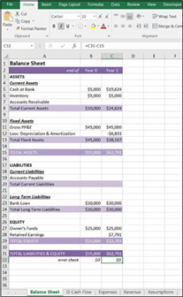
Congratulations! You’ve linked all three financial statements. Check your totals against Figure 10-11 and make sure that you perform a balance sheet error check to see if your total assets equal your total liabilities and equity, and thus balances.
The completed
balance sheet.

 The balance sheet check is the most important one because it’s the most common place where an error will surface due to the many moving pieces that all need to be correct in order for both sides of the balance sheet to balance. Many times, the error will be between the balance sheet and cash flow statement and may be because of an incorrect minus or positive value. When trying to reconcile a balance sheet that does not balance, I find it helpful to remember that the total assets must be equal to the total liabilities and equity, so if I add an item to the assets side of the equation, I need to add an amount of the same value to the other side of the equation.


