
Useful Statistical and Mathematical Functions
Office 2021 includes a range of mathematical and statistical functions, some of which are considered important foundational skills to build more complex formulas.
We will build on prior skills to work with Math & Trig and Statistical functions using Excel 2021 and introduce some additional functions to the mix. We will explore how to generate random numbers using RANDBETWEEN and RAND functions. In addition, we will work through examples of PRODUCT functions, including the SUMPRODUCT, MROUND, FLOOR, TRUNC, AGGREGATE, and CONVERT functions.
In addition, we will investigate the MEDIAN, COUNTBLANK, and AVERAGEIFS statistical functions in this chapter, from which you can experiment and apply to existing or new scenarios when working with workbook data.
The following topics are covered in this chapter:
- Exploring mathematical functions
- Exploring statistical functions
Technical requirements
Prior to starting this chapter, you should be equipped with the knowledge of basic Excel formulas and skills and be able to save files and interact with the Office 2021 environment comfortably. If you have been through prior chapters of this book, you will have the necessary skills to tackle this chapter. The examples used in this chapter are accessible from the following GitHub Uniform Resource Locator (URL): https://github. com/PacktPublishing/Learn-Microsoft-Office-2021-Second-Edition.
Exploring mathematical functions
In previous Excel chapters of this book, we have introduced or built on some mathematical functions such as SUMIF and AVERAGEIFS, so we will not revisit these except to build on existing knowledge or look at other functions within the same family. Let’s start the chapter off by having a look at a few functions to generate random numbers in the next section.
Generating random numbers
In this section, you will learn to understand and apply the RAND and RANDBETWEEN functions to generate random number lists and stop the result from updating in the workbook. We will also look at ways to customize the number range in workbook cells. This function is useful when you need to generate a dataset to test functions with, instead of using your own data. It is also great to generate a random list when training colleagues.
The RAND portion of the function name means random.
The main differences between these two functions are highlighted in the following table:
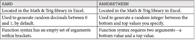
Table 12.1 – Differences between the RAND and RANDBETWEEN functions
We will now look at the syntax of each and how to apply the function in Excel. Proceed as follows:
- Open Microsoft Excel.
- On the first worksheet, select a cell, then start constructing a formula as you would normally.
-
Type =rand.
The process is illustrated in the following screenshot:
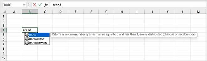
Figure 12.1 – Constructing the RAND function
- Notice the function tooltip displayed on the screen, indicating the result will generate a random number greater than or equal to 0 and less than 1. It also mentions that the function will update when recalculated. This means that every time you update the workbook using the F9 key, the function will update to a different decimal integer.
- Select the RAND function by either double-clicking on RAND in the drop-down list offered or typing ( to continue.
- As we do not have to enter any arguments, simply press the Enter key on the keyboard to see the result.
- When we press the F9 keyboard key, for example, the formula will regenerate when we open the workbook or type into a cell.
-
Should you need a long list of random decimal numbers, simply use the autofill handle to drag the formula down or across to fill in these values. We could also select a range first and then fill the formula. Now that you are familiar with the function, let’s continue with an example to generate a greater range of data.
- Select cells B5:F14, then type =RAND(), as illustrated in the following screenshot, and press Ctrl + Enter to fill the cells:
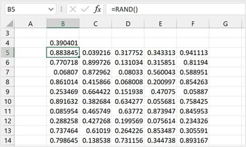
Figure 12.2 – RAND function result
- All the different combinations of decimal values between 0 and 1 are generated within the selected range.
-
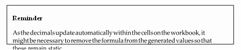
In view of the previous reminder and to make values static within the cells, simply select a range, then right-click and pull the range slightly to the right, then back again to its original position. You should notice a shortcut menu appear with a
list of choices. Select Copy Here as Values Only from the list, as illustrated in the following screenshot:
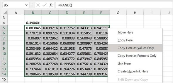
Figure 12.3 – Copy Here as Values Only
- This forces the function to be removed from the cells, leaving behind just the raw data. You can now be confident that the data will no longer update automatically.
Let’s learn how to provide a greater value range when dealing with the RAND function, as follows.
We can expand the range of values the RAND function generates by multiplying by the relevant value. Select cells I5:K5 on the worksheet, then type =RAND()*20. Press the Ctrl + Enter keys when done. Instead of values between 0 and 1 being generated, we can see from the following screenshot that a random list from 0 to 20 is now evident on the worksheet. Note that you can also use a cell reference to multiply by instead:
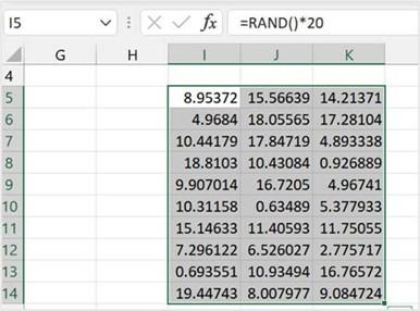
Figure 12.4 – Increasing the value of the RAND default
Whatever the purpose, the RAND function is a quick and easy solution to randomly generate a list of decimals on a worksheet. We can also round these values up or down depending on the requirements. This is covered in the ROUNDUP section in this chapter.
We will now look at one more function to generate numbers automatically.
Learning about the RANDBETWEEN function
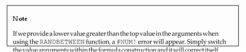
The RANDBETWEEN function is like RAND, except it generates random integers within a bottom and top value constraint you provide. Let’s look at an example, as follows:
- Select cells B18:F26 of the workbook.
- Start typing the formula as follows: =RANDBETWEEN(.
- Notice in the following screenshot that the tooltip is indicating that the syntax requires a top and a bottom argument for this function:
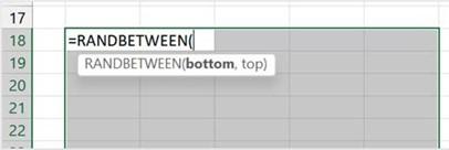
Figure 12.5 – RANDBETWEEN syntax
- Type 45 for the bottom value, then add a comma to separate the arguments. Lastly, enter 580 for the top value.
- Press Ctrl + Enter to generate a list. You will see a list of integers within the bottom and top values entered. The list will update automatically in the workbook. Don’t forget to remove the formula should you not want the list to automatically update.
We will now move on to learn how to multiply ranges together to reach a product in Excel.
Working with PRODUCT functions
In this section, we will explore the PRODUCT and SUMPRODUCT functions.
The PRODUCT function
The PRODUCT function is a simple function that multiplies a given range, ignoring empty cells and any cells that contain text. To work out the Revenue value in the screenshot shown next, we would need to multiply the Cost Per Case value by the Cases Sold value:
- To follow along with this example, open the MattsWinery.xlsx workbook. You can see the syntax here:
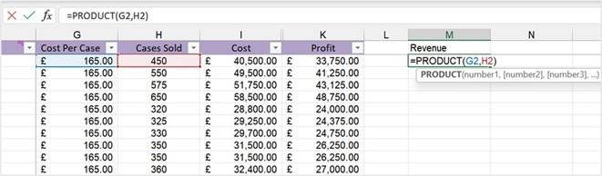
Figure 12.6 – Product syntax
- Click on cell M2, then type =PRODUCT(.
- Enter arguments to multiply the values in the respective cells—namely, G2 and H2—making sure that there is a comma separating the arguments in the formula. Press the Enter key when complete.
- Copy the formula down to the rest of the range to work out the product for all rows in the worksheet.
This method is much easier than the traditional method of multiplying cells using an asterisk to separate arguments. Using the PRODUCT function alleviates any issues with blank cells in the arguments you supply. When we use the asterisk method, and values within the range are missing from the argument, the formula will return a 0 result.
Let’s run through this by way of explanation.
When we use an asterisk to collect cells on the worksheet to multiply, it calculates the product of the cell references added. The process is illustrated in the following screenshot:
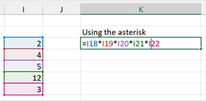
Figure 12.7 – Using the asterisk method
When any of the referred references are empty, the formula returns a 0 result, as illustrated in the following screenshot:
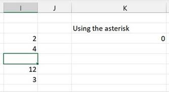
Figure 12.8 – Empty cells causing the formula to return a 0 result
We can, however, use the PRODUCT function in such instances as the function allows cells to be empty as part of the function arguments, as illustrated in the following screenshot:
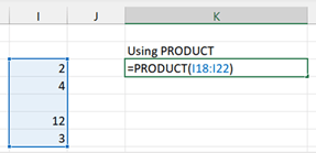
Figure 12.9 – PRODUCT function
When we remove one of the values from the arguments—for example, I20—the formula does not return 0. It will recalculate using the arguments considering the 0 value in I20.
Remember that the PRODUCT function can be implemented along with other functions in the same formula. We will now learn about the SUMPRODUCT function.
The adaptable SUMPRODUCT function
The SUMPRODUCT function can be used to multiply large datasets by multiplying each position in the array. When we use the SUMPRODUCT function, we can be sure that the function will work in any version of Excel. Array functions, as we are already aware, need to be created using the Ctrl + Shift + Enter keys to avoid any array formula output errors. The SUMPRODUCT function is used to create arrays without having to press the Ctrl + Shift + Enter key combination. The SUMPRODUCT function is way more flexible than using COUNTIFS or SUMIFS.
The SUMPRODUCT syntax is shown here:
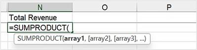
Figure 12.10 – SUMPRODUCT syntax
As you can see from the syntax in the preceding screenshot, the SUMPRODUCT function consists of an array of arguments. The first array argument includes the first range or array to multiply, then sum. The process is repeated for each array argument.
Let’s work through the steps, as follows:
- Open the MattsWinery.xlsx workbook.
-
On the first worksheet, the dataset relates to different wineries and sales data. We will work out the Total Revenue value in cell N2, using the Cost per Case and Cases Sold columns.
- Click into cell N2, then type =SUMPRODUCT(.
- Collect the first range from the worksheet—namely, cells G2:G145.
- Add a comma, then select the next array range, H2:H145.
- Press Enter to see the result of the formula in N2, shown in the following screenshot:
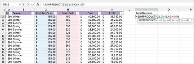
Figure 12.11 – SUMPRODUCT function
- The result displayed in N2 should be 7947624 for the Total Revenue value.
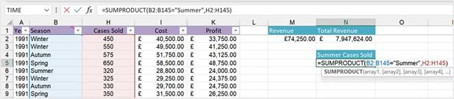
Let’s use the SUMPRODUCT function to sum the total cases sold for the Summer season:
- Using the MattsWinery.xlsx workbook, locate cell N5.
-
The formula we are populating here is very similar to the examples you constructed before, but we will need to tweak the components a little to make it work for us.
We will firstly create a formula incorrectly and then work through how to correct the result.
As we are working out the total number of cases sold during the Summer season, we will be using those columns as arguments in our formula. In cell N5, enter the following formula: =SUMPRODUCT(B2:B145=”Summer”,H2:H145). You can see an illustration of this in the following screenshot:
Figure 12.12 – SUMPRODUCT using SUMIF criteria
- Press Enter to see the formula result. Notice that the result returned is 0. This is due to the first array being represented by true and false values; therefore, we need to force the first array to use 1s and 0s (numeric numbers) instead.
-
This is where the double negative comes into play. We need to force the evaluation of the array to convert from true and false to 0 and 1. Double-click on cell N5 to amend it.
- Type two dashes and ( prior to the first array, like so: =SUMPRODUCT(– (B2:B145=”Summer”),H2:H145).
-
Press Enter to update the result. You should now see a result of 11719 in cell N5.
Similarly, let’s also sum the Amount Owing value for medicines using the
SSGPetFormat.xlsx workbook.
- Click into cell O2, then type the following formula, including the double negative to force the use of 0s and 1s instead of true and false: =SUMPRODUCT(– (L2:L124=”Medicine”),M2:M124).
- The total amount owing for the Medicine category is displayed as £2498.
Use the preceding information to explore the SUMPRODUCT and PRODUCT functions even more by combining them with other functions in the function library. The next section will concentrate on the rounding of values.


