Using DGET to return a single value
- Open the worksheet named Database.xlsx.
-
Notice that the database is formatted as a data table. Make sure that this is the case as we would need the function to update based on any new data being added to the table. The function will be built in cell E3 as this is where we would like to see the formula result returned. In cell D3, we have entered a product named Lighting
– halogen. The contents of this field can be used to locate the retail cost in the database for any product that is entered manually into cell D3.
- Type =DGET( to start the formula.
- Select the database range, in this case, A5:G25. The name of the data table should automatically populate instead of the cell reference at this point. The database table is named Inventory in this workbook, hence the name is now visible in the formula. Ensure that you do have the column headers included in the selection. This is designated by [#All] directly after the table name (refer to the following screenshot example). Insert a comma to move to the next argument.
Figure 10.26 – Formulating the DGET database function
- The next argument we will enter is the field. There are two methods for inserting the field:
-
Identify the column number. In the case of the example, we would insert 6, as
Retail is the sixth column in the worksheet.
-
Include the column header name in inverted commas. Here, we would insert
“Retail”.
-
- Once you have decided which method to use, add another comma to move to the final argument.
- Lastly, we need to select the criteria range. This is the field header and the cell directly beneath it. In this example, we will select cells D2:D3. Make sure D2:D3 is made absolute.
- Press Enter to see the result. Now, change the product to another type to see the retail cost for a different product.
- Should you wish to make the worksheet more efficient, create a validation rule to list the products in cell D3 and then use the drop-down list to choose a product instead.
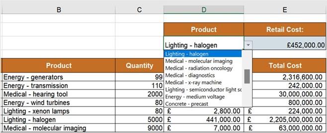
Figure 10.27 – Creating a Product validation rule
Let’s look at a few more examples of database functions.
Constructing DAVERAGE
We will now work out the average gross margin:
-
Click into cell G27 on the DATABASE worksheet (using the Database.xlsx
workbook).
- Construct the formula =DAVERAGE(Inventory[All#],7,$G$2:$G$3) to work out the average gross margin above 50%.
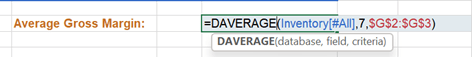
Figure 10.28 – Formula construction for the average gross margin above 50%
- Press Enter to see the formula result of 74.71%. Now we can change the value in cell G3 to see any further updates required.
See whether you can work out the maximum total cost for Division 2, the total quantity sold for Division 1, and the minimum quantity sold for Division 3, using the appropriate function for each. Below is guidance as to the formula you will need to construct and the displayed result for each cell:
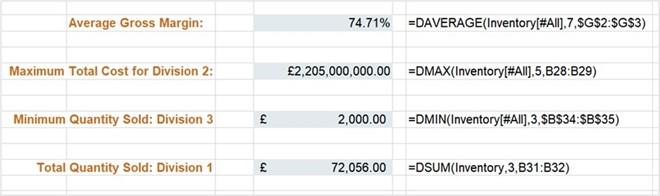
Figure 10.29 – The DMIN, DSUM, and DMAX functions explained
We can expand on our database functions a little more by adding AND/OR criteria. Let’s look at two examples.
Using the AND/OR criteria
In the following steps, we will build a DSUM function to locate the sales figure for the year 1992 and Matts Winery, and with a date range greater than or equal to 01/01/2019 and less than or equal to 31/12/2020:
- Continuing with the Database.xlsx workbook, make sure you have clicked on the MULTIPLE CRITERIA worksheet.
- The database table is located in cells A1:I145. To build the AND criteria, we will include the column headers along with the relevant criteria in the same row.
- Click into cell K1 and then add the columns and criteria as per the following table:

Table 10.6 – Columns and criteria to get ready for the DSUM function
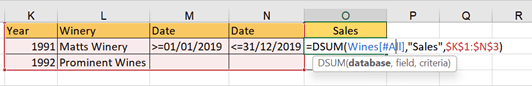
- We are now ready to construct the formula in cell O2.
- Type =DSUM( and then select the database range A1:I1445, including the headings. Insert a comma to move to the next argument.
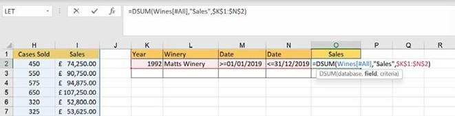
Figure 10.30 – DSUM formula construction
-
The field argument we are returning values from is the Sales column. Either type a 9
for the column number within the database range, or “Sales”.
- Lastly, select the column headings and their criteria in cells K1:N2. Don’t forget to make the range absolute.
- Press the Enter key to see the sum of sales for Matts Winery and the year 1992 and between the date range 01/01/2019 and 31/12/2020.
- We will now add another row to the criteria table to include the OR criteria.
- As we would like to locate the sales for Matts Winery 1991 between the date range listed, OR prominent wines for 1992, we would need to amend the year in K2 to 1991. In K3, add the year 1992 and Prominent Wines in cell L3.
- Lastly, amend the formula in cell O2 to include the second row in the criteria selection so that it includes the OR criteria.
Figure 10.31 – OR condition DSUM formula
- Press Enter to update the formula in O2.