
Using the COUNTIFS statistical function
In our previous edition book, Learn Microsoft Office 2019, we learned all about the COUNTIF function. Let’s look at an example to recap this function, and explore the COUNTIFS function at the same time.
Recapping the COUNTIF function
In the next topic, we will expand on prior knowledge and discover how to resolve two sets of data by locating missing data by comparing two tables. There are, of course, many methods (functions and tools) to achieve this type of scenario in Excel. In this example, we will use COUNTIF to achieve this:
- Open the workbooks named RECON1.xlsx and RECON2.xlsx to follow along with this example.
- Locate the first worksheet in the RECON1.xlsx workbook. On this sheet, we have a list of wines and sales, including a WV No column (for the wine ID). We have recently had a huge number of workbooks transferred from our previous drive and notice that we seem to be missing some data and have located a second workbook (RECON2.xlsx) with similar data. To compare these two workbooks, we will use the COUNTIF function.
- Click into cell I2 as we will construct the formula here. In our previous edition book, we learned about syntax and looked at examples of the COUNTIF function. We will therefore not recap this here.
- Type =COUNTIF( to start the construction of the formula.
- The range we are looking at to see whether WV No exists is located in the RECON2. xlsx workbook, so we need to navigate to the workbook and collect the range from the WV No column (excluding the column heading). Select cells A2:A137. Note that if we were selecting a range in the same workbook to compare, we would need to apply absolute referencing to the range. Moving to an external workbook, as in this example, has automatically applied the absolute referencing to the range.
- Press the comma to move to the next argument.
- Navigate back to the RECON1.xlsx workbook to select the criterion. The criterion is A2.
- Press Enter to see the result in the first instance and then use the AutoFill handle to fill the formula to the rest of the column to compare the results in the two tables.
-
If the Missing Data column reflects a 1, this means that the data is matching in both tables. A 0 would indicate that the data exists in table 1 (RECON1.xlsx), but not in table 2 (RECON2.xlsx).
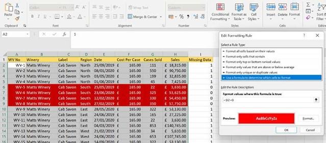
- We can go one step further and apply conditional formatting to highlight the cells on the worksheet that are evident in the RECON1 workbook, but not in the RECON2 workbook.
- Select the range A2..H145 in the RECON1 workbook, and then select Home | Conditional Formatting | New Rule | Use a formula to determine which cells to format.
-
Enter the following formula in the Format values where this formula is true: field:
=$I2=0. Apply a format of your choice and then click on OK and OK again to apply the rule. The rows that exist in table 1, but not in table 2, are highlighted on the worksheet.
Figure 10.32 – Conditional formatting applied to indicate rows that are missing from table 2
- Note that you have to have both workbooks open for the COUNTIF formula to populate. Not having the workbook open will report a #VALUE! error in the cell
– this means that the reference to the workbook is not found and therefore it is prompting you to open the workbook for the formula to work.
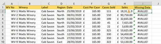
Figure 10.33 – #VALUE! error indicating the formula cannot populate due to the associated workbook being closed
If we wanted to find the missing data in the second workbook by reconciling it with the first workbook, we can perform this action by repeating the process from the second workbook to the first.
Now that we have mastered reconciling data using the COUNTIF function, we will learn to apply the COUNTIFS function. The IFS functions were introduced in this chapter in a previous topic.
Learning the COUNTIFS statistical function
The second example is to introduce the COUNTIFS function. The difference between the
COUNTIFS and COUNTIF functions is as follows:
- The COUNTIF function counts the number of cells within a range that meet a single condition you specify.
- The COUNTIFS function counts the number of cells by evaluating different criteria in the same or different ranges.
Let’s look at an example using COUNTIF:.
- Open the workbook named COUNTIFS.xlsx.
- The workbook contains a dataset related to wines and sales. We would like to find out how many cases of wine were sold per region. This is a simple formula to construct, but remember it can have multiple criteria and criteria ranges.
- In order to pull information from the main dataset, we need to copy the relevant column headings and paste them onto the worksheet so that we can exact the data and build the formula. We also need to add the criteria for each. Make sure you have the following column headings and criteria starting in cell K1:
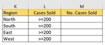
Figure 10.34 – Copied column headings and criteria
-
In cell M2, construct the following formula:
=COUNTIFS(E2:E145,K2,H2:H145,L2),K2,H2:H145,L2)
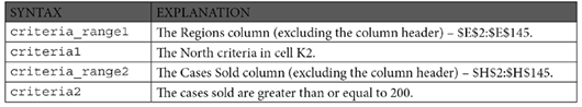
Table 10.7 – Syntax and explanation for COUNTIFS
- Do not forget to copy the formula using AutoFill to the rest of the cells in Column M of the worksheet. Here is a representation of the result and formula result:
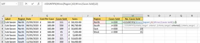
Figure 10.35 – The COUNTIFS function showing criteria and selected worksheet ranges
You are now able to construct the COUNTIFS function, and collect ranges and criteria on the worksheet to locate the number of cases sold per region that are greater than or equal to 200. To populate the formula to show all the cases sold less than or equal to 150, or any other criteria, simply amend the values in the Cases Sold column to reflect the change.
Summary
You now have theoretical knowledge about formula construction, and should feel confident to perform calculations adhering to certain rules. You are able to construct, edit, and evaluate dynamic arrays as a result of understanding the terms and when to use the function. During the chapter, you have mastered the building of IFS functions and built on the VLOOKUP function by adding the IFERROR and MATCH functions. We explored the new XLOOKUP function, its syntax, and general error returns, and constructed the XMATCH and INDEX functions, too.
We learned about the forgotten database functions and explored working with multiple conditions. Lastly, we recapped the COUNTIF function and worked through examples using COUNTIFS.
In the next chapter, we will explore date functions and look at some more statistical, logical, and mathematical functions, including SWITCH, Subtotals, and SUMIF. In addition, a large part of this chapter will be devoted to PivotTable customization.


