
Removing spaces or hidden characters
There are several ways to remove spaces from workbook data once it’s been imported. We can use the TRIM and CLEAN functions, SUBSTITUTE, or even the Flash Fill command. The following table lists these functions and some syntax examples:
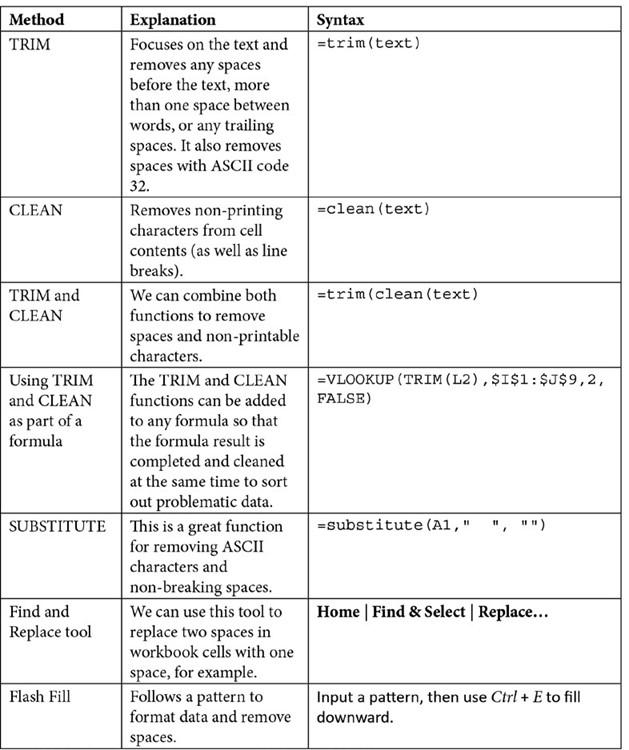
Table 9.2 – Cleaning data by removing spaces from data
- Open the workbook named Spaces.xlsx.
-
Notice that the existing data contains additional spaces before some text, such as
B13. Trailing spaces are difficult to visually detect within datasets.
- Let’s use Flash Fill to clean data. We can use this command to fix the case, as well as copying a pattern to fill in the email addresses, combine data, and remove spaces.
- Click into cell D2 and simply type the format you need the cell data to be represented with. Then, press the Enter key:
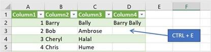
Figure 9.47 – Flash Fill shortcut key, Ctrl + E
- Press Ctrl + E to place the data in the rest of the cells, based on the pattern you provided in D2. In this instance, it will fix any space issues, as well as joining the name and surname together into one column. Always check that the data is consistent and that you receive the result you require:
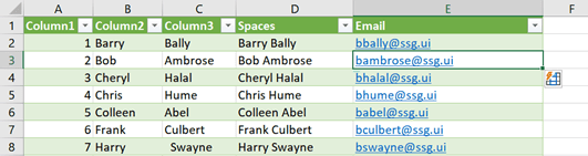
Figure 9.48 – Flash Fill to expand email addresses
- Notice that the Flash Fill icon appears in the bottom-right corner of a cell, along with a drop-down list of options to choose from.
- If we want to add email addresses for each of our employees, we can type the email pattern for the fi st employee into cell E2, then press Ctrl + E to fill the rest of the cells.
- Flash Fill can also be used to correct the case of the text. Type BARRY BALLY into cell F2, then use Ctrl + E to fill the contents down. This is a great way to correct text that has been imported with a mix of upper and lowercase letters.
The next few functions we will explore can be applied separately or jointly to data. Here, we will look at the TRIM, CLEAN, and SUBSTITUTE functions. Follow these steps:
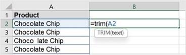
- Open the workbook named Trim.xlsx.
- Click inside cell B2, then type =trim(A2):
Figure 9.49 – The TRIM function
- Press Enter to confirm, then double-click the AutoFill handle to copy the formula down the column.
- Additional spaces will be removed from the text.
-
Now, let’s try the CLEAN function. Cell B20 contains text that has a line break. This function is used to remove non-printing and line break characters. Click inside cell B20, then type =clean(B20).
-
Press Enter to confirm. The line breaks in this example have been removed from
the text, but you will notice that the spaces still exist. To fix this, we can use CLEAN
and TRIM together.
- Delete the formula in cell B20, then replace it with =trim(clean(B20)):
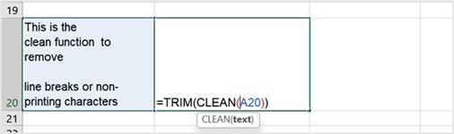
Figure 9.50 – Using the TRIM and CLEAN functions together
- The SUBSTITUTE function will remove spaces or non-breaking spaces too. We can use the SUBSTITUTE function to replace a certain character type with another.
-
Cell A23 contains text as well as an accent character, ^. We would like to remove this character from the text. Before we do this, we will need to locate the ASCII character number code for ^. In this case, if we locate Insert | Symbols
| Symbol, we can locate the ^ character, then find the code at the bottom of the dialog box. The code for the ^ character is 94. Now that we know the code for the ^ character, we can use this in our formula. Click inside B23 and type
=substitute(A23,CHAR(94),””):
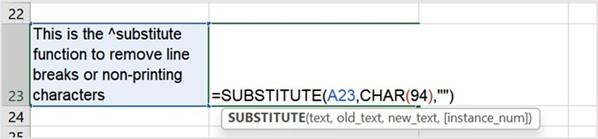
Figure 9.51 – Using the SUBSTITUTE function to replace characters
- Press Enter to confirm this, after which the text will be formatted correctly without the accent.
At times, we need to remove data that has been duplicated in the worksheet. We will address this in the next section.


