
Extracting using wildcard characters
Wildcard operators are useful for extracting data according to a partial match within a cell. For instance, if the Winery column listed names of wine farms and we wanted to filter all the cells containing the text wine, we could search the Winery column for the partial match using *wine. The asterisk represents any number of characters – in this case, any number of characters before and after wine. Let’s get started:
- Select the WINERY worksheet. We will filter the Winery column so that all the wineries containing the word wine are extracted to the Wildcards worksheet.
- The range N1:02 contains the filter criteria headings, namely Winery and Profit. Enter *wine in the Winery field.
- Enter the following criteria:
- List range: A1:K145
- Criteria range: N1:O2
- Copy to: A1 of the Wildcards worksheet
- List range: A1:K145
- Click the OK button to display the results of the filter.

Now, we will look at the new filter and sort functions.
The previous section explained how to use the Advanced Filter. However, there is a much quicker way to get results using new functions available in Office 2021.
Extracting using the FILTER function
The first new function is the FILTER function. The syntax for this function is as follows:
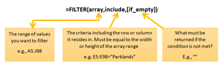
Figure 9.29 – Syntax for the FILTER function explained
To follow along with this example, open the workbook named SSGNewFunctions. xls:.
- The workbook contains headings from A4:J4. To use the FILTER function to achieve the output we require, the column headings need to be duplicated to the results area of the worksheet.
- Copy the content of A4:J4 and paste it into cell L4 so that it extends from L4:U4.
-
In cell L5, enter the following formula to filter all the Parklands data only:
=FILTER(A5:J98,E5:E98=”Parklands”,”Other”)
- Press Enter. The data has been filtered to the new location:
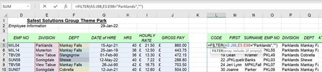
Figure 9.30 – FILTER function showing the results of the formula
- If data is updated in the existing range dataset, then the filtered list will update too. The updated list – for example, in L5 in the previous example – is called spill.
- We can evaluate the formula using the F9 key. Double-click to edit the formula in cell L5 on the worksheet. Highlight the include part of the formula:
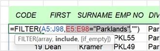
Figure 9.31 – Highlighting the include part of the formula
- Press the F9 key to evaluate the result.
- Here, we can see that the results correspond with the source data in column E, which is true for each instance of Parklands:
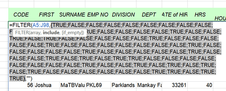
Figure 9.32 – Pressing F9 to evaluate the formula
- We can also filter to another worksheet. Simply copy the headings from the first worksheet to the second worksheet of this workbook, namely Shewe.
- In this example, we will spill all the employees from the Shewe department who have a gross pay greater than 600. As we are using the AND criteria for this example, we will need to use parentheses around each separate criteria with an asterisk in between them.
- Click inside cell A2 of the Shewe worksheet.
-
Enter the following formula:
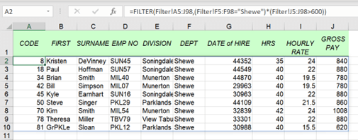
=FILTER(Filter!A5:J98,(Filter!F5:F98=”Shewe”)
*(Filter!J5:J98>600)).
- Press Enter to confirm and update the worksheet:
Figure 9.33 – Result of the AND filter condition showing the formula in the formula bar
- Here are a few tips for other methods of working with the filter criteria:
-
If we were using an OR criteria instead of AND, we would substitute * with a
+ sign.
-
If we were filtering a department that is not in the list, we could specify the error return result for the missing department in the list and include a no result return for each of the columns in the table.
- Using the previous example, we can set up a filter to locate the Slipslide department and return the text not found if the item is not located in the column; that is, =filter(Filter!A5:J98,Filter!F5:F98=”Slipslide”, “not found”).
-
The downside of this is that it will only include the text that wasn’t found for the first cell:
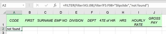
Figure 9.34 – Filter showing not found for one cell of the range
If we wanted to display results for each cell, we would simply change the parentheses to curly parentheses and list all the cell contents within. Here is an example:
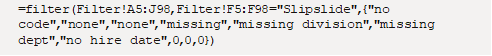
The following screenshot shows the output:
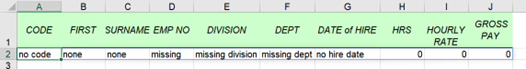
Figure 9.35 – Result showing that the criteria do not match each cell in the range
The final tip is to select only the columns you would like a result from as the array. Include the CHOOSE function directly after the FILTER function to specify the columns to include in the array. Experiment with these functions to apply them to your specific working environment.
In the next section, we will review conditional formatting and master conditional formatting based on the formula.


