Restricting and Validating Data
After you finish building a financial model, you may be tempted to keep it to your- self, because you don’t want anyone to mess up your formulas or use the model inappropriately. Models should be collaborative, but you need to build your model in such a way that it’s easy for others to use and difficult to mess up. One great way of making your model robust for others to use is to apply data validations and pro- tections to the model. This way, the user can only enter the data he’s supposed to.
For a practical example of how to use data validation, let’s take the Project Cost- ings Analysis from the “Absolute cell referencing” section earlier in this chapter (refer to Figure 6-6). Your colleague is using the model you’ve built and he can tell by the way in which cell D3 has been formatted (with shading) that you expected people to make changes to it. He’s not sure anymore how many days this project is going to continue, so he types TBA into cell D3 instead. As soon as he types TBA, that really messes things up! As you can see in Figure 6-16, the formulas you’ve already built were expecting a number in cell D3, not text.
Instead of allowing the user to put anything into any cell, you can change the properties of this cell to allow only numbers to be entered. You can also change it to allow only whole numbers or numbers in a given range.
Follow these steps:
- Download File 0601.xlsx from www.dummies.com/go/financialmodeling inexcelfd
and select the tab labeled 6-17.-
Select cell D3.
-
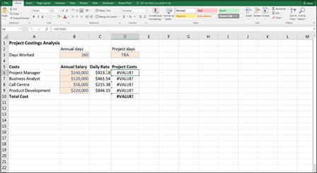 FIGURE 6-16:
Text in an input causing errors.
-
Go to the Data tab on the Ribbon and press the Data Validation icon in the Data Tools section (see Figure 6-17).
The Data Validation dialog box appears (refer to Figure 6-17).
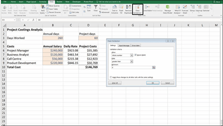 FIGURE 6-17:
Using data validation to restrict entry into cells.
- On the Settings tab, in the Allow drop-down list, select Whole Number; in the Data drop-down list, select Greater Than; and in the Minimum fi enter 0.
Now only allow whole numbers greater than zero can be entered into cell D3. Try entering text such as TBA. Try entering a negative value. Excel won’t allow it, and an error alert will appear.

 If you want, you can enter a warning message on the Input Message tab of the Data Validation dialog box. For example, you might want the following message to appear: “Warning! Only enter numerical values.” On the Error Alert tab, you can enter another message that appears if someone ignores the warning and tries to enter invalid text. I’m usually tempted to type something mischievous, such as: “Invalid entry. Your hard drive will now be completely erased.”
Creating drop-down boxes with data validations
Not only does the data validation tool stop users from entering incorrect data into your model, but you can also use it to create drop-down boxes. In the Data Valida- tion dialog box, from the Allow drop-down list, select List, as shown in Figure 6-18. In the Source fi enter the values you’d like to appear in the list with a comma between them such as Yes, No. A simple drop-down list is created in cell B12 with only two options: Yes and No. The user can’t enter anything else.
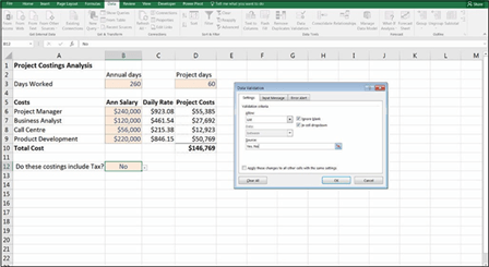 FIGURE 6-18:
Using data validation to create a simple drop-down list.
 No one can enter a value in a cell that goes against your data validation rules, but it’s still possible to paste over a cell that is restricted by data validation. In this way, users can inadvertently (or deliberately) enter data into your model that you did not intend.
You can also create a drop-down list that links to existing cells within the model. For example, in Figure 6-19, I don’t want the users to include a region that is not included in the list shown in column F. So I’ve used a data validation list, but instead of typing in the values (which would be very time-consuming), I can link to the range already containing the regions — $F$2:$F$5 — which is a much quicker way of inserting a drop-down list.
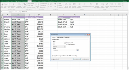 FIGURE 6-19:
Using data validation to create a linked,
dynamic
drop-down list.

 Because I’ve linked the drop-down list, this drop-down is now dynamic. If some- one edits any of the cells in the range F2:F5, the options in the drop-down list will automatically change.
You can also add protection to your model by going to the Review tab on the Rib- bon and clicking the Protect Sheet button in the Changes section. Enter a pass- word if you want one, and click OK. This will protect every single cell in the entire worksheet, so no one will be able to make any changes at all! If you want users to be able to edit certain cells, you’ll need to turn off the protection, highlight those cells (and only those cells you want to change), go to the Home tab on the Ribbon, and click the Format button in the Cells section. Deselect the Lock Cell option that appears in the drop-down list. Turn the protection back on again, and only the cells that have been selected will be unlocked.
 Keep in mind that it’s reasonably easy to crack an Excel password (search the Internet for Excel password cracker), so if someone wants to get in and make changes to your protected model, he can. I recommend that you treat Excel pass- words as a deterrent, not a definitive security solution.
Goal Seeking
Another tool that’s very useful for financial modeling is goal seek. If you know the answer you want, but you want to know what input you need to achieve it, you can work backward using a goal seek.
In order to run a goal seek, you must have
» A formula
» A hard coded input cell that drives this formula
It doesn’t matter how complicated the model is. As long as there is a direct link between the formula and the input cell, the goal seek will calculate the result correctly.
 The input cell must be hard coded. It won’t work if the input cell contains a formula.

Limiting project costs with a goal seek
What a goal seek is and how it works is best demonstrated using a simple model. For a practical example of how to use a goal seek to limit project costings, follow this series of steps as shown.
Again, let’s take the Project Costings Analysis from earlier in the chapter (refer to Figure 6-6). As shown in Figure 6-20, I’ve used simple formulas to calculate the total cost of a project based on the number of days worked, giving a total costing of $146,769. Unfortunately, however, I’ve only budgeted for $130,000 in staff costs. If I want the project to come in under budget, I need to know how much I need to cut the days worked by. I can manually tweak the number of days that has been input in cell D3, but it would take a long time to get the number exactly right. By using a goal seek, I can do it in seconds:
-
On the Data tab of the Ribbon, in the Forecast section, select What-If Analysis and then select Goal Seek.
The Goal Seek dialog box (shown in Figure 6-20) appears.
-
In the Set Cell fi make sure the cell contains the outcome you want,
the total cost in cell D10.
-
In the To Value fi enter the number you want D10 to be, $130,000.
-
In the By Changing Cell fi enter the cell you want to change, the
project days in cell $D$3.
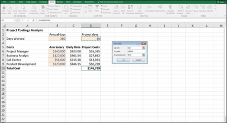 FIGURE 6-20:
Using a goal seek to limit project
costings.
-
Press OK.
The number of project days in cell D3 automatically changes to 53.1446540880503, which is a lot more information than you probably need! Round it down manually, by typing 53 into cell D3, which will change the total costings so that they come just under the $130,000 target you needed.
 If you tried to manually enter a number with decimal places into cell D3, the data validation you created earlier in this chapter in Figure 6-6 would not allow it. Because a goal seek is essentially pasting the number into the cell, it circumvents the data validation rule, as though you had copied and pasted the value.
Calculating a break-even point with a goal seek
Using goal seek is also very helpful for break-even analysis. In this section, you perform a simple break-even calculation using a goal seek. (For more detail on break-even analysis, see Chapter 9.)
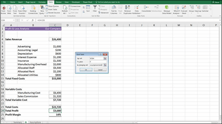
For a practical example of how to use a goal seek to calculate a break-even point, let’s work with the model you built earlier in this chapter. You’ve linked it through in such a way that if the number of units sold changes, the revenue changes, and so does the variable costs. You’d like to know the minimum number of units you need to sell in order to cover costs (the break-even point). Follow these steps:
- Go to the Assumptions worksheet, and try changing the number of units sold from 8,940 to 8,000.
-
Go back to the IS worksheet, and you’ll see that the profi has
dropped from 20% to 14%.
You could continue to do this manually until you reach zero, but a goal seek will be much quicker and more accurate.
-
On the Data tab on the Ribbon, in the Forecast section, select What-If Analysis and then select Goal Seek.
The Goal Seek dialog box appears (see Figure 6-21).
- In the Set Cell fi enter the cell that contains the outcome you want (the profi C24.
- In the To Value fi enter the number you want C24 to be, 0.
-
In the By Changing Cell fi enter the cell you want to change (the
number of units on the Assumptions page), $A$3.
 FIGURE 6-21:
Using a goal seek to calculate a break-even point.
-
Press OK.
The number of units in cell A3 on the Assumptions page automatically changes
to 6,424, which is the break-even point.


