
Connecting to and Transforming Data
So far, we have learned about the basics of the Power BI interface. However, to truly unlock the power of Power BI, we need to expand our data model. To do that, in this chapter, we will learn about the Power Query Editor and how to relate multiple tables of data to one another to create a more complex data model. Every good visual report starts with a good data model, so we must learn how to properly ingest, transform, and load our data into Power BI.
The following topics will be covered in this chapter:
- Getting data
- Transforming data
- Merging, copying, and appending queries
- Verifying and loading data
Technical requirements
You will need the following to follow the instructions in this chapter:
- An internet connection.
- Microsoft Power BI Desktop.
- Download LearnPowerBI_CH4Start.pbix and the Budget and Forecast.xlsx, People and Tasks.xlsx, and Hours.xlsx files from GitHub at https://github.com/PacktPublishing/Learn-Power-BI- second-edition/tree/main/Chapter04.
- Check out the following video to see the Code in Action: https://bit. ly/3bVTQwc
Getting data
Power BI is all about working with and visualizing data. Thus, we must incorporate some additional data into our model. In Chapter 2, Planning Projects with Power BI, we covered the data and data sources that Pam required and would be using. To emulate this data, we will use Excel files, so ensure that you have the Excel files from this chapter’s Technical requirements section downloaded and that your LearnPowerBI.pbix file is open in Power BI Desktop.
In this section, you will create your first query and then add some additional data to your data model.
Creating your first query
To determine whether or not Personal Time Off (PTO) should be approved, it is important to understand where the company is concerning budgets and forecasts. Whether or not the company, department, and/or location is on target in terms of its budget can be an important consideration when approving or denying time off.
Unlike the calendar table from Chapter 3, Up and Running with Power BI Desktop, where we used DAX to create a calculated table, this time, we will import data into our data model using a query. A query is simply a series of recorded steps for connecting to and transforming data
To create a query, follow these steps:
- In Power BI Desktop, choose Get Data from the Home tab of the ribbon. Note the default list of potential data sources and select More… at the bottom of the list:
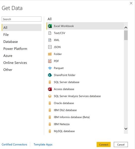
Figure 4.1 – The Get Data section
There are over 150 default connectors available for ingesting data. These connectors are broken down into several categories:
All: This lists all of the available connectors.
- File: File connectors, including Excel, text/CSV, XML, JSON, folder, PDF, and SharePoint folders.
- Database: The Database section lists sources such as SQL Server, Access, Oracle, IBM DB2, IBM Informix, IBM Netezza, MySQL, PostgreSQL, Sybase, Teradata, SAP, Impala, Google BigQuery, Vertica, Snowflake, Essbase, and AtScale.
- Power Platform: Power Platform includes Power BI datasets and dataflows, as well as Dataverse.
- Azure: Azure lists many different services, such as Azure SQL Database, Azure Synapse Analytics, Azure Analysis Services, Azure Blob Storage, Azure Table Storage, Azure Cosmos DB, Azure Data Lake Storage, Azure HDInsights (HDFS), Azure HDInsights Spark, Azure Data Explorer (Kusto), Azure Databricks, and Azure Cost Management.
- Online Services: There is a substantial collection of online services, including Microsoft technologies such as SharePoint Online, Exchange Online, Dynamics 365, Common Data Service, DevOps, and GitHub, as well as third parties such as Salesforce, Google, Adobe, QuickBooks, Smartsheet, Twilio, Zendesk, and many others.
- Other: other connectors include Web, OData, Spark, Hadoop (HDFS), ODBC, R, Python, and OLE DB.
You can also regard connectors as specific and generic:
- Specific connectors connect to proprietary technologies, including IBM DB2, MySQL, Teradata, and many more.
- Generic connectors are included under the Other category and support connecting to any technology that supports industry standards, such as ODBC, OData, web (HTML), and OLE DB. Because there are hundreds, if not thousands, of data sources that are not specifically listed that support these standards, there is an almost unlimited number of data sources that can be connected to within Power BI.
At the bottom of Figure 4.1, there are two links. The first is a link that reads Certified Connectors. One of the reasons Power BI has so many data source connectors available is because Microsoft has created the ability for customers and third parties to extend the data sources supported by Power BI through custom connectors.
By default, Power BI only allows connectors that have been certified through Microsoft’s certification process to be used in Power BI. This can be changed by going to File | Options and settings | Options, selecting Security, and then
adjusting Data Extensions. Custom connectors are placed in the Power BI Desktop installation folder, under the [Documents]\Power BI Desktop\Custom Connectors folder. This folder was created after installing and running Power BI.
The second link is for Template Apps. Template Apps are prepackaged dashboards and reports that can be connected to live data sources. Clicking the
Template Apps link opens a web browser window or tab connected to the Power BI Apps marketplace.
-
Click back on the All category and select the first item in the list; that is,
Excel Workbook.
- Browse to your Budgets and Forecasts.xlsx file and click Open. The dialog that’s displayed is known as the Navigator:
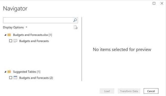
Figure 4.2 – The Navigator dialog
For Excel files, the Navigator dialog will list all the pages and tables within the Excel file. The suggested tables are the areas in Excel that are specifically marked as tables.
- Click the checkbox next to Budgets and Forecasts and observe that a preview of the data is loaded in the right-hand pane:
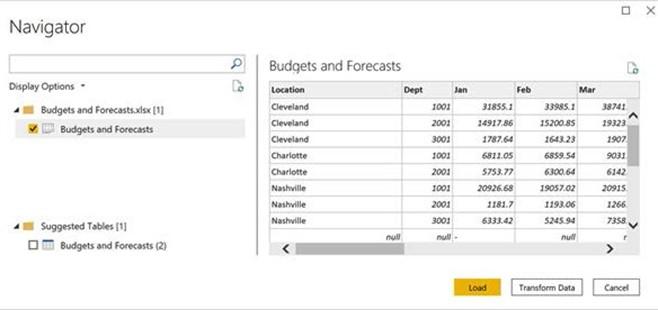
Figure 4.3 – Navigator dialog with a preview of the data
Note that three buttons are available at the bottom of the page: Load, Transform Data, and Cancel.
- Click the Load button. Once the loading dialog completes, click on the Data view and then the Budgets and Forecast table to see this data loaded into the data model:
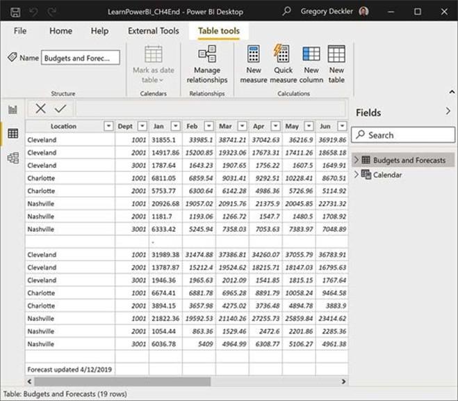
Figure 4.4 – Budgets and Forecast table
The data that’s displayed represents the budget and forecast information for our fictional professional services firm. Behind the scenes, Power BI created a query and attempted to make intelligent decisions about the data, including identifying column names and data types.
Congratulations! You have created your first Power BI query!
Getting additional data
Let’s get some additional data. Since we are tracking PTO for people, we need to get some data about the employees at the company, as well as the tasks that they are performing.
To get this data, perform the following steps:
- From the Home tab of the ribbon, choose Get Data and then Excel workbook.
-
Choose the People and Tasks.xlsx file and click the Open button. The Navigator
dialog will be displayed, as shown in the following screenshot:
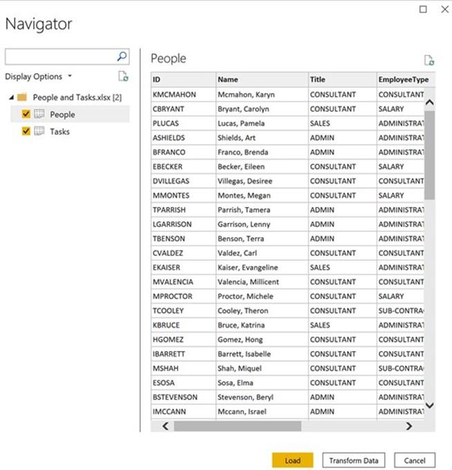
Figure 4.5 – Creating queries for People and Tasks
-
As shown in the preceding screenshot, check both the People and Tasks pages and click the Load button.
While exploring this data back in the Data view of Power BI Desktop, we can see that we now have two additional tables: People and Tasks.
The People table contains information about the employees of the company. By looking at the People table, we can see that we have information such as ID, Name, Title, EmployeeType, TermDate, HireDate, and Location.
The Tasks table contains information about the projects or tasks that employees work on and whether or not those tasks are billable. In the Tasks table, we can see that there is TaskID and Category in the first row, but we can also see that these are not our column names. Not to worry; we will fix that later when we transform this data.
The final data that we need is the actual hours that employees are working. To do this, perform the following steps:
- Click on the Home tab of the ribbon, choose Get Data, and then Excel workbook.
- This time, choose the Hours.xlsx file and click the Open button.
- In the Navigator dialog, this time, just choose January and click Load.
Now that we have loaded all of our data, we can move on to transforming the data as necessary. As you become more familiar with Power BI, you will likely choose the Transform Data button instead of the Load button while you are importing data.
Transforming data
While Power BI did a good job of automatically identifying and categorizing our data, the data is not entirely in the format required for analysis. Therefore, we need to modify how the data gets loaded into the model. In other words, we need to transform the data. To do that, we will cover using a powerful sub-application known as Power Query Editor.
Touring the Power Query Editor
Similar to how we provided a tour of Power BI Desktop in Chapter 3, Up and Running with Power BI Desktop, this section provides a tour of Power Query Editor. Power Query Editor can be launched from the Home tab by choosing Transform data in the Queries section of the Ribbon. Once launched, the following screen will be displayed:
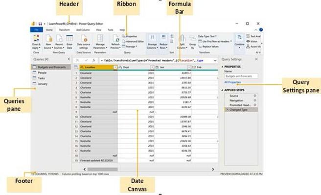
Figure 4.6 – Power Query Editor
As you might expect, the Power Query Editor interface is similar to, and shares common elements with, Power BI Desktop. The Power Query Editor user interface is comprised of eight main areas. Refer to the preceding screenshot while reading about these eight areas in the subsequent sections.
Header and Quick Access Toolbar
Nearly identical to Power BI Desktop, the Header is the small strip at the top of the Power Query Editor window. This area is standard for Windows applications. Left-clicking the application icon in the left-hand corner provides the standard sizing and common exit commands, such as Minimize, Maximize, and Close.
Next to this icon is the Quick Access Toolbar. This toolbar can be displayed above or below the ribbon, and commands within the ribbon can be added to this toolbar by right-clicking an icon in the ribbon and selecting Add to Quick Access Toolbar.
By default, only the Save icon is displayed.
To the right of the Quick Access Toolbar is the name of the currently opened file and next to that is the name of the application, Power Query Editor.
Queries
The Queries pane displays a list of the various queries associated with the current Power BI file. As queries are created, those queries are displayed here. This area also allows you to group queries, as well as any errors that are generated by data rows within queries.
Query Settings
The Query Settings pane provides access to properties for the query, such as the name of the query. By default, the name of the query becomes the name of the table within the data model.
More importantly, the Query Settings pane includes a list of Applied Steps for a query. A query is just a series of applied steps, or transformations, of the data. As you transform the data that’s been imported by a query, a step is created for each transformation. Thus, executing a query to refresh data from a data source is just a matter of re-executing these steps, or using transformation operations.
Data Canvas
Data Canvas is the area within Power Query Editor where a preview of the data that’s been loaded into the model is displayed. This area is contextual, displaying the data table for the currently selected step of a query. This area is similar to the Data view within Power BI Desktop and is the main work area for viewing and transforming data within queries.
Footer
The Footer area is contextual and is based on what is selected within Power Query Editor. Helpful information, such as the number of rows and columns in a table and when the last preview of the data was loaded, is displayed here.
Ribbon
Below the title bar is the Ribbon. Users who are familiar with modern versions of Microsoft Office will recognize the function of this area, although the controls that are displayed will be somewhat different. The ribbon consists of six tabs:
- File: The File tab displays a fly-out menu when clicked that allows Power BI Desktop files to be saved, as well as Power Query Editor to be closed, and changes made within Power Query Editor to be applied.
- Home: The Home tab provides a variety of the most common operations, such as connecting to sources and managing parameters and common transformation functions, such as removing rows and columns, splitting columns, and replacing values.
- Transform: The Transform tab provides data manipulation functions that let you transpose rows and columns, pivot and unpivot columns, move columns, add R and Python scripts, and many scientific, statistics-related, trigonometry, date, and time calculations.
- Add Column: The Add Column tab provides operations that focus on adding calculated, conditional, and index columns. In addition, many of the functions that are available from the Transform tab are also available in this ribbon.
-
View: The View tab includes controls for controlling the layout of the Power Query interface, such as whether or not the Query Settings pane is displayed, and whether the formula bar area is displayed.
- Help: The Help tab includes useful links for getting help with Power BI, including links to the Power BI Community site, documentation, guided learning, training videos, and much more.
Formula bar
The Formula bar allows the user to view, enter, and modify the Power Query (M) code. The Power Query formula language, commonly called M, is a functional programming language comprised of functions, operators, and values. M is the underlying data connection and transformation technology for Microsoft Power Automate, PowerApps, Power BI Desktop, and Power Query in Excel
M is the language behind queries in Power BI. As you are building a query in Power Query Editor, behind the scenes, this is building an M script that executes to connect to, transform, and import your data. In reality, each of the applied steps in a query is a line of Power Query M language code. You do not need to worry about that just yet, but we will explore this in the Merging, copying, and appending queries section.
Transforming budget and forecast data
Now that we have connected to our data, we need to perform some transformation steps to clean up the data and prepare it for our data model. To do this, follow these steps:
-
In the Power Query Editor window, select Budgets and Forecasts from the
Queries pane on the left.
Looking at the data, we can see that we have a blank row in the middle and several extraneous rows at the end. Looking at the column headers, we can see that
Power BI has identified that our first row contains column names and has already categorized our columns as text (ABC), whole numbers (123), and decimal (1.2). The table contains columns for Location, Department, and then a column for each month. As we scroll horizontally to the end, we can see a column called Type.
-
In the Query Settings pane, under APPLIED STEPS, we can see that some steps have already been applied to our query. These steps were automatically created by Power BI.
A query is just a collection of applied steps. If we click on these steps, we can see how our query changes our data table at each step.
-
Clicking on the Navigation step, we can see that our column headers are labeled
Column1, Column2, and so on.
- When we click on the Promoted Headers step, we can see that the first row has been promoted to be column headers, but that all of our columns are labeled ABC123.
- Clicking on the Changed Type step, we can see that this is where our columns are categorized according to their data types.
Now that we understand how applied steps transform the data, let’s apply some of our transformation steps!
Cleaning up extraneous bottom rows
Let’s clean up those extraneous rows at the end. To do that, follow these steps:
- Ensure that the last step, Changed Type, is selected in the Query Settings pane.
-
From the Ribbon, select the Home tab and then the Remove Rows button in the
Reduce Rows section. Select Remove Bottom Rows:
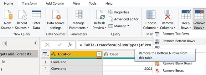
Figure 4.7 – Removing rows
- In the following dialog, type 2 and then click the OK button:
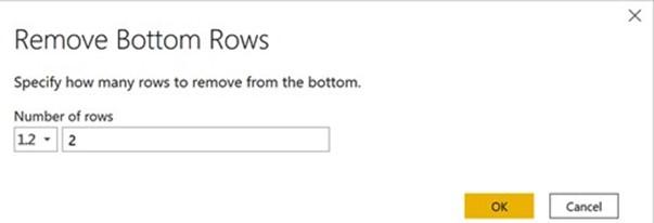
Figure 4.8 – Remove Bottom Rows dialog
Observe that the last two rows have been removed from the Data Canvas and that an additional step, Removed Bottom Rows, has been added to the bottom of our query steps in the APPLIED STEPS area of the Query Settings pane
Filtering rows
Now, let’s clean up that mostly blank row in the middle, row 9. To do this, follow these steps:
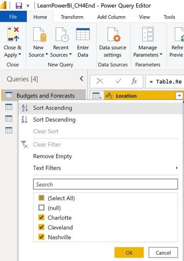
- In the Location column header, click the drop-down arrow and you will notice that there are several options, including sorting, text filters, and a search bar. The Text Filters area presents several useful text filtering options, including filters such as Equals, Does Not Equal, Begins With, Does Not Begin With, Ends With, Does Not End With, Contains, and Does Not Contain. Also, note that all of the distinct values that appear in the column are listed, including (null), Charlotte, Cleveland, and Nashville. As datasets become larger, you may see a List may be incomplete warning message. This occurs because Power Query Editor samples the first 1,000 rows of data. If you see this message, you can click on the Load more link to have Power Query Editor analyze all the rows of data:
Figure 4.9 – Filtering rows
- As shown in the preceding screenshot, uncheck the box next to (null) and then click the OK button.
Notice that the row of null values in the data table has been removed and that a new step has been added to the query called Filtered Rows in the APPLIED STEPS area of the Query Settings pane. Also, notice that a small funnel icon appears in the Location column’s header button, indicating that this column has been filtered.
Unpivoting data
Let’s put this data into a better format for analysis. Since the numeric data that we will need to analyze appears in multiple columns (the month columns), this will make analysis difficult. It would be much easier to analyze if we transformed this data so that all of the numeric data was in a single column. We can do this by unpivoting our month columns. To unpivot our month columns, perform the following steps:
- Start by selecting the column header for Jan.
- Scroll horizontally to the right until you see the last column, Type.
- Hold down the Shift key and then select the column header labeled Dec. Now, all of the columns between and including Jan through Dec will be highlighted in yellow and selected.
-
Click on the Transform tab and choose Unpivot columns from the Any Column
section of the Ribbon:
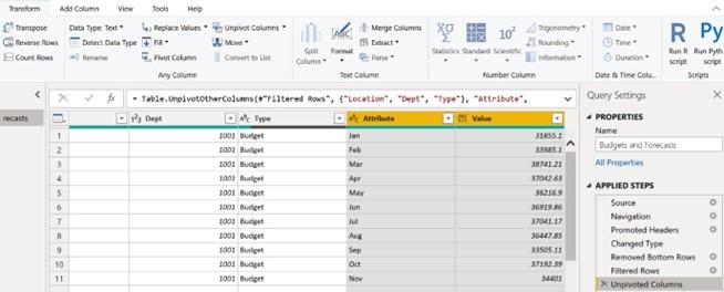
Figure 4.10 – Unpivoting columns
As shown in the preceding screenshot, our month columns have been transformed into two columns called Attribute and Value. Our former column names, Jan, Feb, Mar, Apr, May, and so on, now appear as row values under the Attribute column, and our numeric values appear in a column called Values. The Unpivoted Columns step appears in our APPLIED STEPS area.
-
Double-click the Attribute column header and rename this column Month.
A Renamed Columns step will appear in the APPLIED STEPS area of the Query Settings pane.
Unpivoting data is a common operation with Excel-based data as spreadsheets are generally designed for easy data entry. However, having multiple columns for the same data element is almost always a bad idea for data analysis in Power BI.
Using Fill
Now, we want to fix our Type data. Notice that the Type column contains spotty information. The first 12 rows contain the word Budget, and then there is a gap until row 97, where the next 12 rows contain the word Forecast, and then another gap. We
want all of these rows to contain either Budget or Forecast. To fix the data, we will use the
Fill functionality by performing the following steps:
- Select the Type column, then right-click and choose Fill, and then Down.
- Notice that our Type column now contains a value for each row and that a Filled Down step appears in the APPLIED STEPS area of the Query Settings pane.
The Fill operation takes the latest value found in the column and replaces any blank or null values with that value until a new value is found. Then, this operation repeats.
Changing data types
In the data table, notice that our Value column is categorized as general data. As shown in Figure 4.10, we can tell this by the ABC123 icon that appears in the Value column header. The ABC123 label means that the values in the column can be either text or numeric. To fix the data type, perform the following steps:
- Click the ABC123 icon in the column header of the Value column and choose Fixed decimal number. The ABC123 icon is replaced by a $ and a Changed Type1 step is added to the APPLIED STEPS area of the Query Settings pane.
-
Similarly, click the 123 icon in the Dept header and change this to Text. Notice that the 123 icon is replaced with an ABC icon and that the values in the column are no longer italicized and are left-justified versus right-justified. While our department codes may be numeric, we do not want to ever sum, average, or otherwise aggregate these values numerically, so changing them to be treated as text makes sense. Notice that a new step was not added to the APPLIED STEPS area of the Query Settings pane. Since our last step in the query was already a step to change the data type of
a column, this new operation for the Dept column was simply added as part of the current Changed Type 1 step.
Changing data types also affects the sort order, so sometimes, leaving the data type as numeric and using a default summarization of don’t summarize can also be effective.
Transforming People, Tasks, and January data
Now, let’s move on to ensuring that our other tables are ready for analysis. In the following sections, we will perform similar operations on the People, Tasks, and, and January queries as we did in the Transforming budget and forecast data section.
Transforming the People query
To transform the People query, perform the following steps:
- In Power Query Editor, click on the People query in the Queries pane. Notice that four steps have already been created in this query: Source, Navigation, Promoted Headers, and Changed Type. Power BI has automatically added several query steps to make the first row the column names and identify the data types of the columns. The first four columns – that is, ID, Name, Title, and Employee Type – have all been identified as text (ABC). The next two columns, TermDate and HireDate, have a calendar icon. These are date columns. The final column, Location, is a text column (ABC).
- Ensure that all of these columns have the correct data type. If not, change their data type by either clicking on the data type icon in the column header or choosing the Transform tab of the Ribbon and using the Data Type dropdown in the Any Column section. When you are finished, your data types should be the same as the ones shown in the following screenshot:
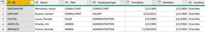
Figure 4.11 – Column data types for the People query
These are all the transformations required for the People query. Now, let’s move on to the
Tasks query.
Transforming the Tasks query
To transform the Tasks query, perform the following steps:
-
In Power Query Editor, click on the Tasks query in the Queries pane. Notice that there are only three APPLIED STEPS in this query: Source, Navigation, and
Changed Type. There are two columns named Column1 and Column2. Also, note that the first row contains the TaskID and Category values. We want the values in this first row to be the names of our columns.
- Click the Navigation step in the APPLIED STEPS area of the Query Settings pane.
- Click the Transform tab and choose Use First Row as Headers, the second icon from the left. An Insert Step message will be displayed, asking you to confirm that you wish to insert a step into the query:
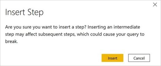
Figure 4.12 – Insert Step dialog
- Click the Insert button. Notice that a Promoted Headers step has been inserted between the Navigation step and the Changed Type step. Our column headers are now TaskID and Category.
- Click on the Changed Type step and notice that an error is displayed. This is because the Changed Type step was referring to the columns as Column1 and Column2, but now, these columns are called something different.
- Remove the Changed Type step by clicking on the X icon to the left of the step name.
- Now, change the data types of both columns to Text by either clicking on the data type icon in the column header (ABC123) or choosing the Transform tab of the Ribbon and using the Data Type dropdown in the Any Column section.
The transformations for the Tasks query are now complete. The next query to transform is the January query.
Transforming the January query
Moving on to the January query, perform the following transformation steps:
-
In Power Query Editor, click on the January query in the Queries pane. Note that four APPLIED STEPS exist: Source, Navigation, Promoted Headers, and Changed Type.
The EmployeeID, TaskID, JobID, Division, TimesheetBatchID, TimesheetID, and PayType columns are all Text columns (ABC).
The Date, PeriodStartDate, and PeriodEndDate columns are all Date columns (calendar icon).
The Hours, HourlyCost, HourlyRate, TotalHoursBilled, and TotalHours columns are all decimal number (1.2) columns.
- Make sure that the Changed Type step is selected and then change HourlyCost and HourlyRate to Fixed decimal number by either clicking on the data type icon in the column header (1.2) or choosing the Transform tab of the Ribbon and using the Data Type dropdown in the Any Column section. A Change Column Type prompt will be displayed each time. Choose the Replace current button each time, as shown in the following screenshot:
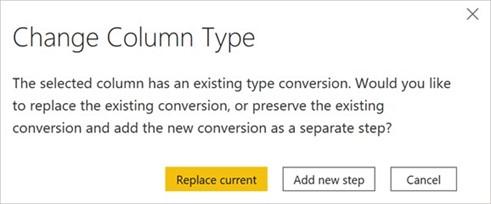
Figure 4.13 – Change Column Type dialog
This finishes the basic transformation work we must perform on our queries. However, we have not finished transforming our data yet. We will now move on to more complex data transformations.


