
Setting up a conditional formatting rule
Now that we have the rule in place, we would like to ensure that every time a user selects an item from the drop-down list from a single cell in column L, the color of the row changes accordingly. Remember that you don’t need to set the validation rule to create the conditional formatting rule; it just helps in terms of data entry/user error. Let’s get started:
- Select the data you wish to apply a conditional formatting rule to. Do not select your headings, just the data you wish to apply the format to.
- Since we are creating a rule that’s a little more complex than the existing rules offered in the drop-down categories, we need to go to Home | Conditional Formatting | New Rule….
- Select Use a formula to determine which cells to format.
- Using the service categories and color table as a guide, we will add a formula for two of the categories – that is, Follow Up Consult and Medicine. If you prefer, you can add all the categories, but we will only set up two for now.
- Click inside the field under the Format values where this formula is true heading.
- Type =$L2=”Follow Up Consult”:
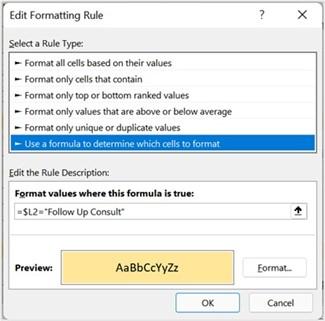
Figure 9.40 – Using a formula to determine which cells to format
Note that not using the correct cell reference in the formula would cause the rule to apply formatting to the incorrect cell data. If you have applied conditional formatting to cells and then apply formatting to the rows manually, the conditional format may return the incorrect row selection as a result.
- Click the Format… button to select the appropriate color, then click OK to confirm, then OK again to return to the Conditional Formatting Rules Manager screen.
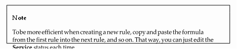
- Click New Rule… to create the next rule. Repeat this step for each of the values and colors you require.
- Once the rules have been set up with their respective color coding, click the OK
button to apply these to the workbook. You will see some changes right away:
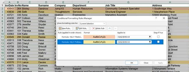
Figure 9.41 – Conditional Formatting Rules Manager
- If you need to make amendments to any of the rules, remember to select the entire dataset again, then go to Home | Conditional Formatting | Manage Rules….
- Double-click on the rule you wish to amend in the Conditional Formatting Rule Manager dialog box. Alternatively, select a rule and then click Edit Rule… to make amends.
Conditional formatting formula rules can become quite creative, depending on the scenario and results you require. We can use any function to construct a conditional format rule, just like you would if constructing a formula within workbook cells.
Let’s look at another example containing a more complex formula:
-
Open the workbook named CondFormatISNAVlookup.xlsx. The workbook has been set up to analyze two sets of data to determine which customers are listed in the first set of data, but not the second. A logical test has been set up to display the text Not found in Table 2 if the customer is missing from the dataset in Table
2. We would like to add color to the entire row when the customer is not evident in the second dataset.
- Select the A3:L29 range, then go to Home | Conditional Formatting | New Rule….
Select Use a formula to determine which cells to format. Enter the following formula in the Format values where this formula is true field:
=(ISNA(VLOOKUP($A3,$A$33:$L$57,1,FALSE))).
- Click the Format button, then select a Fill color of your choice to apply to the rows on the worksheet that meet the criteria.
- Click on the OK button, then OK again to exit and return to the worksheet. The customers (rows) that appear in the first table, but not in the second table, will be highlighted on the worksheet:
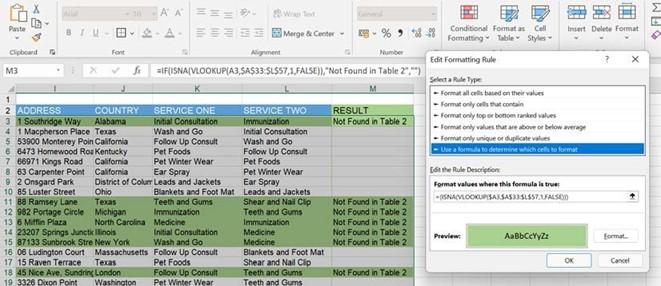
Figure 9.42 – The result of using the Conditional Formatting rule once the formula criteria have been entered
Using Icon Sets
In addition to conditional formatting rules, we can also apply Icon Sets to indicate whether certain conditions have been met in the dataset to add visual impact. Icon sets could include values, text entries, or based on a formula, to mention a few. Let’s take a look at an example:
- Open the workbook named Wines.xlsx to follow along. We will apply icon sets to the Cases Sold column to visually indicate the status.
- Select cells H2 through H145, then navigate to Home | Conditional Formatting.
- Predefined icon sets are available via the Icon Sets category. Here, select the applicable style from Directional, Shapes, Indicators, or Ratings, or click More Rules… to customize the visual markers.
- Click More Rules….
- Notice that Format all cells based on their values is selected under the Select a Rule Type heading.
- Under the Edit the Rule Description heading, select Icon Sets for Format Style.
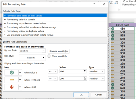
- Select an icon set of your choice – for this example, we will select the seventh style in the list.
-
Customize each icon to your requirements. For this example, we will leave the first icon set to the green check symbol. The second icon we will amend to the yellow dash icon, and the third to a red down arrow.
- Amend the Value column as follows:
- Green check symbol when value is >=400
- Yellow dash when value is <400 and >=200
- Red down arrow when <200
- Green check symbol when value is >=400
- Change the Type column to reflect Number:
Figure 9.43 – Applying icon sets to data
- Click OK to apply the icon sets to the data in column H. Once the data has been updated, the icon sets will adapt accordingly.
You should now be confident in customizing icon sets. See whether you can experiment with the Formula option from the Type drop-down list. In the next section, we will learn how to get data ready when importing from external sources into Excel.


