
New Features, Filters, and Cleaning Data
In the previous edition of this book, we concentrated on all the basic skills concerning data entry, including being able to distinguish between spreadsheet elements, as well as the various output options. In this chapter, you will learn about essential updates for, and the new features of, Excel 2021. You will learn all about Advanced Filter and the new FILTER
function, as well as more about conditional formatting rules. We will focus on cleaning data and learning how to import, clean, join, and separate data while learning about some of the new features of Excel 2021 along the way, such as the UNIQUE function.
In this chapter, we will cover the following topics:
- New features to enhance proficiency
- Using Advanced Filter
- Conditional formatting functions
- Importing, cleaning, joining, and separating data
Technical requirements
To complete this chapter, you must have an understanding of the purpose of spreadsheets and be proficient at locating and launching Excel 2021. If you have worked through the previous edition of this book, you will already be familiar with the interface elements and the various setting options, constructing a workbook, applying formats, filtering data, and creating charts.
The examples for this chapter can be found in this book’s GitHub repository at https:// github.com/PacktPublishing/Learn-Microsoft-Office-2021-Second-
Edition.
New features to enhance proficiency
In this section, we will look at the exciting new features of Excel 2021 for desktop and any enhancements that have been made to existing features. We will also explore some of the new and/or existing feature updates for Excel for the web.
Unhiding multiple sheets
When using the new version of Excel, we can now unhide more than one sheet at a time. To follow along, use the file named SSGThemePark-Hide.xlsx:
- Select the second, third, and fourth sheets in the workbook.
- Right-click on the worksheet tabs, then select Hide.
- To unhide hidden worksheets in one go, right-click on the Employees sheet and select Unhide… from the menu.
-
Select all the worksheets using the Shift + click keyboard keys, or individually select sheets using Ctrl + click:
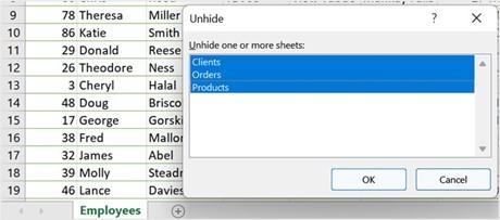
Figure 9.1 – Unhiding multiple worksheets at the same time
- Click OK to confirm this.
Troubleshooting tip
If you need to provide your specific build of Excel when troubleshooting features, you can share this information easily with your support agent or community. To do so, visit File | Account | About within the Excel environment, then right-click and copy the build number from the top of the screen. This way, you won’t have to write this information down and re-type the details when you want to share them. Remember to always share personal data responsibly and within the correct channels:
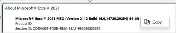
Figure 9.2 – Copying build information to share when troubleshooting
Collaborating using Sheet View
As we learned when we covered the Word and PowerPoint topics in this book, collaboration has been greatly enhanced with modern commenting and co-authoring. At a glance, we can see who is editing a workbook by looking to the top right of it. Everyone who has been invited to the shared workbook can add comments and work in real time.
Sheet View is a new feature in the latest version of Excel that allows files to be shared using a separate view so that when we are collaborating and manipulating data using filters, the source data is not affected. Only changes to data within the actual cells will be saved to the underlying shared workbook. The only constraint is hiding and showing rows when you’re using the desktop version of Excel with Sheet View turned on. Hiding or showing rows will update in the Default view, not Sheet View, even though you can hide or show rows in Sheet View.
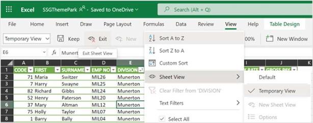
- Select View | New to create a new Sheet View:
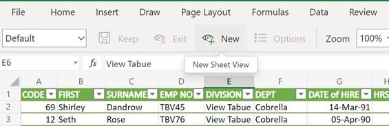
Figure 9.3 – New Sheet View
-
You will notice that the view is created as a temporary view, as shown on the left of the ribbon. Use the drop-down arrow to the right of Temporary View to see the
Default view (this is the source file). When clicking on a column header to filter, the Sheet View list is also evident here:
Figure 9.4 – Exit Sheet View
-
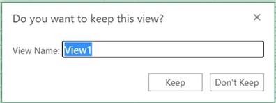
While making changes to the data, such as filters and sorts, you are not obstructing anyone else who has shared a status on the file. Once you have finished manipulating the data to suit your requirements, you can Exit the Sheet View, after
which you will be prompted to confirm whether you would like to Keep the view by naming it. Alternatively, you can choose Don’t Keep:
Speak Cells
Figure 9.5 – Prompt to Keep or Don’t Keep Sheet View
At times, you may be working from a printed hardcopy, but need to check certain cells and compare them to your worksheet data. Although Speak Cells is not a new feature, it is often overlooked and can be very useful. Let’s take a look:
- Visit the QAT and navigate to the drop-down list to select More Commands….
- From the Excel Options dialog box, select Quick Access Toolbar.
- Select All Commands from the Choose commands from drop-down list.
-
In the list, locate Speak Cells, then click the Add >> button to move the selection to the right-hand side of the pane. Do the same with Speak Cells – Stop Speaking Cells so that you can control when the feature is enabled or disabled:
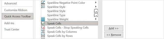
Figure 9.6 – Adding Speak Cells to the QAT
- Click OK when you’re done.
- To activate Speak Cells, select an area on the worksheet, then click the Speak Cells button on the QAT. The worksheet cells will speak back to you. To disable this feature, click the Speaking Cells – Stop Speaking Cells button:
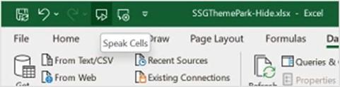
Figure 9.7 – Speak Cells button added to the QAT


