VLOOKUP and HLOOKUP
The lookup functions — VLOOKUP and HLOOKUP — are very often used in build- ing financial models and are often the “go to” function for many modelers and analysts.
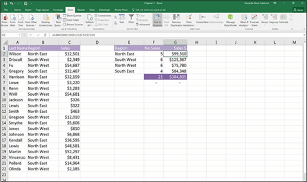 FIGURE 7-28:
The completed
sales total table.
Despite its popularity, the humble VLOOKUP is often misused and overused because many users — especially when they’re just starting out — don’t understand exactly how it works. VLOOKUP stands for vertical lookup. It can be used any time you have a list of data with a unique lookup field in the leftmost column. The VLOOKUP function searches through a data set and returns a corresponding match from a specified row and column.
HLOOKUP works in exactly the same way, except that the data is horizontally orientated instead of vertically oriented.
Mapping Data with VLOOKUP
Using the previous example from the last section, you have a list of sales and regions. Let’s say you want to abbreviate the region names from “North West” to “N/W,” because that’s what your team is used to seeing.
If you followed along with the last example, simply insert an extra column before column D to enter the abbreviation as shown in Figure 7-28. Right-click column D, and select Insert. Or you can download File 0701.xlsx at www.dummies.com/go/
financialmodelinginexcelfd. Open it and select the tab labeled 7-29.
To solve this problem, follow these steps:
-
In cell G2, start to enter the abbreviations for each region.
This is the mapping table you’re using to map the regions to their abbreviated names. If you’re using Excel 2013 or later, Flash Fill will begin to automatically populate the data for you as shown in Figure 7-29. Very cool.
- Select cell C2 and then click the Insert Function command on the Formulas tab (or just press Shift+F3).
-
In the Select a Function box, scroll down until you see the VLOOKUP
function; select VLOOKUP and click OK.
-
The fi parameter is the criteria you’re testing — in this case, the fi region you need the abbreviation for, North East — so enter B2 in the Lookup_value fi
The next fi is the table array, which contains the data you want to reference. This is where it gets tricky. The criteria you’re looking for must always be in the far-left column of the data table you’re referencing in the table array.
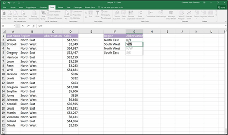 FIGURE 7-29:
Using Flash Fill.
-
In the Table_array fi enter F2:G5, because in this case, the data you’re
referencing will be in that range.

Press the F4 shortcut key to lock the cell reference.
 In the Col_index_num fi you need to enter which column the value is found
in. You need to tell the function which column in the table array you want it to return. In this case, you want it to tell you the abbreviation for the region. So, counting from the far-left side of the table array (starting in column F), you want it to return to the second column.
-
Enter a number 2 in the Col_index_num fi as shown in Figure 7-30.
The optional fourth fi Range_lookup, is where you specify whether a close match is okay.
-
If you want an exact match, enter zero in the Range_lookup fi
otherwise, leave it blank.
You may also enter TRUE or FALSE, but typing a zero or leaving it blank is
 quicker.
Make sure to enter a zero or FALSE in the last fi If you leave it blank, it will search for a “close” match and return an incorrect result. There are very few instances where you want a close match.
-
Click OK to complete the formula.
The completed formula will be =VLOOKUP(B2,$F$2:$G$5,2,0) with a returned result of “N/E.”
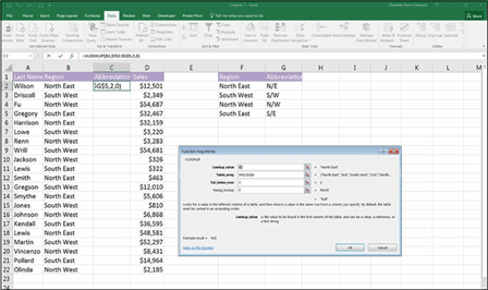 FIGURE 7-30:
The VLOOKUP
Function Arguments dialog box.
- Copy cell C2 all the way down the column and compare your results to Figure 7-31.
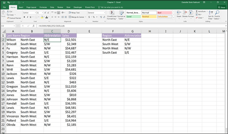 FIGURE 7-31:
The completed report with
region
abbreviations.
-
Go to the mapping table and adjust the abbreviated names.
For example, change “N/E” to “NE,” and you’ll notice the abbreviations in column C also automatically change. In this way, you can save time in building your reports.
Breaking a VLOOKUP
If you’ve created a VLOOKUP in a model such as the one in the preceding section, this should work well . . . until someone enters or deletes a column in your source data! A formula such as the following specifically asks for the second column, so it won’t work if someone inserts a column range within the Regions range:
=VLOOKUP(B2,$F$2:$G$5,2,0)
It won’t work because your required column becomes the third column, but the VLOOKUP is still asking for the second.
 VLOOKUPs are not very robust formulas — you can see how easy they are to break! Here’s what you can do to avoid this problem and make your VLOOKUP more robust:
 » Protect the sheet to stop people from inserting or deleting rows or columns.
» Use a “helper” row where the column number needs to be manually updated,
or automatically calculated with a COLUMN function.
» Insert an error to alert the user if this mistake has occurred.
» Replace the hard-coded number 2 with a dynamic function such as a COLUMN or MATCH function that will automatically update.
Using the HLOOKUP function
The HLOOKUP works in exactly the same way as the VLOOKUP, except that the data is arranged horizontally instead of vertically. The HLOOKUP function is sub- ject to exactly the same issues as VLOOKUP and it works in exactly the same way, except for the orientation. If your source data in the range is orientated vertically, use VLOOKUP, and if it’s orientated horizontally, use HLOOKUP. See the nearby sidebar for a practical example of using an HLOOKUP nested formula in a financial modeling context.
 WORKING WITH NESTED FUNCTIONS
As you may have discovered by now, Excel allows you to include more than one func- tion in a formula. For example, you can multiply a sum total by another number with the following formula:
= SUM(B1:B20)*A3
But this does not make it a nested formula. A nested formula is a function that’s included inside another function. This technique allows you to build more complex for- mulas. For example:
=IF(SUM(D3:D23)<0,1,0)
This is a basic IF statement, but a SUM function has been included in one of the
fi
The IF statement is probably most commonly used as a nested function. You can actually nest up to 64 functions within a formula model, but this is not recommended, and it’s certainly not good modeling practice!
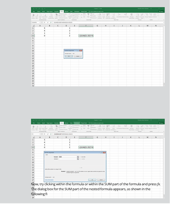
With most functions covered in this chapter, I encourage you to make use of the Function Arguments dialog box. This dialog box doesn’t work easily with nested formulas, but there is a bit of a trick to it.
Try typing in the nested formula:
=(SUM(D1:D5)*AVERAGE(A1:A5))/12
Try to go into the Insert Function dialog box by pressing the fx button next to the Formula Bar. An unhelpful Function Arguments dialog box appears, as shown in the following fi
