Using Audit Tools to Find and Correct Errors
When inheriting a model, there are several factors to come to grips with: the layout, design, formatting, assumptions, and formulas. Of all these, following the formula calculations is the most difficult, and verifying and validating formulas can be very time-consuming. The fastest way to understand a formula when you see it for the first time is to go into Edit mode. Double-click a cell, or select it and press F2. If the formula’s source inputs are on the same page, they’ll show visually where the source data is coming from that feeds the cell calculation, as shown in Figure 5-5. The color codes are helpful; each range in the formula will be the same color as the highlight source data that feeds it. If you’d like to try this out for yourself, down- load File 0501.xlsx from www.dummies.com/go/financialmodelinginexcelfd. Open it and select the tab labeled 5-5.

 When you’re in Edit mode and you decide that you need to change the range the formula is referring to, you can use the mouse to click and drag the colored lines to reference a different cell. For example, in Figure 5-5 if you wanted the range B3:B12 to be A3:A12 instead, click the colored line showing between the A and B column and drag it so that the cell reference is column A instead of column B.
On the Formulas tab in the Ribbon, there is a formula auditing section that con- tains a number of tools that you’ll find useful when trying to understand someone else’s financial model. Just remember that using these audit tools in Excel is not the same as performing a formal financial model audit.
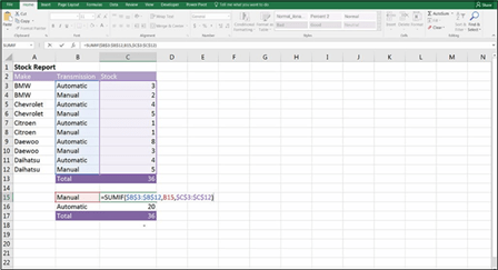 FIGURE 5-5:
Using Edit mode to see formula
inputs.
 A formal financial model audit is a very detailed process in which a model auditing team takes the model apart and checks it meticulously for errors. If the bank is lending you money based on the results of the financial model, one of the condi- tions of the loan might be that the model be audited to make sure that the results can be relied upon. Getting a model professionally audited can be an extremely expensive undertaking, but it’s really the only way to ensure that there are no errors. Note that a financial model audit is sometimes called a model review to dif- ferentiate it from a financial audit.
Of course, creating your own financial model is a lot more interesting than check- ing someone else’s. But Excel’s audit tools make checking someone else’s model somewhat easier. Formula errors are the most common type of error in financial models, and the audit tools exist almost solely for the purpose of finding these formula errors.
The formula auditing tools can help get to the root of what’s causing the error in a cell through tracing relationships among cells within your worksheet. These tools will help you find the source of an error, but they’ll also, more important, help you find an error you didn’t know was there. By tracing the relationships, formula auditing lets you test formulas to see the precedents (cells that directly supply the formulas) and the dependents (the cells that depend on the results of the formulas). Excel also offers a way to visually reverse any potential sources of an error in the formula of any particular cell.
The formula auditing tools can be found in the command buttons located in the Formula Auditing group on the Formulas tab of the Ribbon. These command but- tons include the following:
» Trade Precedents/Trace Dependents: In trying to understand a model, you’ll spend the majority of your time working through the formulas and making sure you understand exactly how each output has been calculated. Trace
Precedents and Trace Dependents are good places to start when you’re trying to see where the cell links are coming from and going to. These tools are helpful to identify the linkages that exist between the cells and display the relationships visually with blue tracer line arrows.
To use Trace Precedents, start with an output cell that contains a formula you want to understand, such as the formula =SUM(B3:B7) in cell B8 in Figure 5-6. Select the cell and click the Trace Precedents button in the Formula Auditing section of the Formulas tab. This displays blue tracer line arrows, which show which cells B8 depends on.
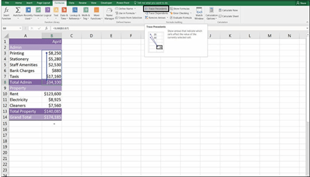 FIGURE 5-6:
Trace Precedents.
 Using the same cell, you can see which cells, in turn, depend upon B8 by using Trace Dependents, as shown in Figure 5-7.
 Click the Trace Precedents or Trace Dependents button again, and it goes further and shows the precedent of the precedent, or the dependent of the dependent.
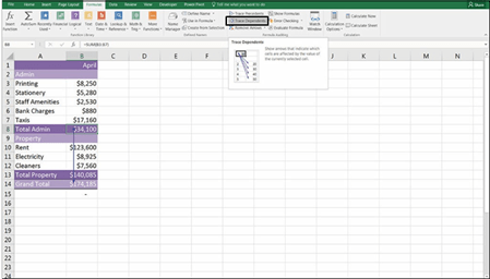 FIGURE 5-7:
Trace Dependents.
If the source data is located on another sheet, instead of the blue tracer line arrow, a black dotted line appears with the worksheet icon, as shown in Figure 5-8.
Cells that are the cause of errors will show as red tracer arrows instead of blue. When the cell links to external fi the source fi must be open so that the Formula Auditing tool can trace these dependencies.
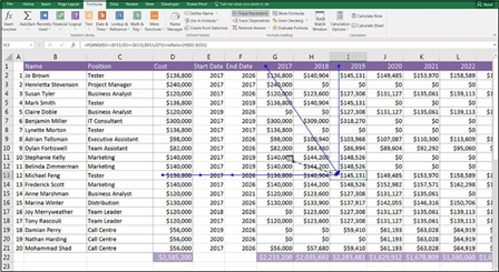 FIGURE 5-8:
The black dotted line indicates a
link to an off-sheet source.
 The tracer lines disappear when the fi is saved. You can manually remove them by clicking Remove Arrows under the Trace Dependents button on the Ribbon. Make sure you remove the arrows before printing the sheet; other- wise, they’ll show up in the printed document.
You can also jump to precedent cells by using these shortcuts:
- Ctrl+[ to jump to and highlight precedent cells
- Ctrl+] to jump to and highlight dependent cells
- Ctrl+G or F5 and then Enter to return to the previous cell
DEALING WITH REDUNDANT ASSUMPTIONS
A common problem in fi models, particularly “legacy models” that have been around for a long time and have been passed on from one staff member to another, is that inputs and assumptions may exist that aren’t actually being used in the model’s calculations. Redundant assumptions can happen when modelers need to use source information that is already in the spreadsheet and re-create it without realizing that they’re entering a duplicate set of assumptions or data. Often, as a model evolves, parts of the model calculations are deleted, but the assumptions that fed into those calcula- tions remain, despite the fact that they’re no longer needed. Using the Trace Dependents formula auditing tool is the easiest way to see if any formulas are linking to an input cell. This tool will allow you to trace forward and backward throughout the model.
One technique you can use to remove redundant cells is to color-code all the input assumption and calculation cells. Then go to the model outputs and trace back the formu- las, using trace precedents and trace dependents. As each input assumption is validated, change the color of the input cells back to their original color. At the end of the process, if any cells are still colored, you’ll know that they’re redundant and they can be deleted.
When removing redundant inputs from a model, delete entire rows or columns by right- clicking and selecting Delete Row or Delete Column instead of selecting the cell and pressing Delete. This way, if the deletion had been linking to a formula, you see an
error. Clearing cells simply changes the value to zero, which won’t necessarily return an error and can cause undetected errors to remain in the model.
Formula auditing doesn’t always show up if certain tools such as data tables, array for- mulas, and the INDIRECT and OFFSET are relying on that cell. For this reason, make sure you save before deleting any redundant assumptions in your model and check the output of the model for #REF! or other errors before continuing. If removing the cells has caused an error, you can simply undo or close without saving to revert to the version of the fi prior to the changes.
Of the tools that are contained within the Formula Auditing section of the Formu- las section on the Ribbon, Trace Precedents and Trace Dependents are most likely to be the most useful. There are a few other tools, however, which also warrant a mention.
» Evaluate Formula: Another way of checking formulas is to actually take them apart using the Evaluate Formula tool. This tool is most useful with long and complex nested formulas because it evaluates each part of the formula
separately in the current cell that you’re in, as shown in Figure 5-9.
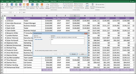 FIGURE 5-9:
The Evaluate Formula tool.
 You can also evaluate a partial formula manually by selecting a part of the formula and pressing F9. You have to select an entire section of the formula that makes sense in its own right; for example, in a nested formula such as
 =IFERROR(IF(E3<$F$1,-E3/D3,0),0), shown in Figure 5-10, you can select this portion of the formula: E3<$F$1. If you then press F9, the result of that portion of the formula alone will be displayed as a value, which in this case is FALSE. You can see that the statement being evaluated is false, so the “value if true” part of the formula will be the result of the statement, rather than the “value if false.” (For more information on using IF statements, see Chapter 7.)
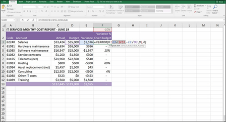 FIGURE 5-10:
Auditing part of the formula manually.
» Error checking tools: If you make a mistake — or what Excel thinks is a mistake — a green triangle will appear in the upper-left corner of the cell. This
happens if you omit adjacent cells, such as the error that is shown in Figure 5-11, or if you enter an input as text that looks like it should be a number.
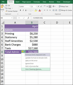 FIGURE 5-11:
Error checking.
In this instance, Excel provides a very helpful notifi that the formula in cell B8 does not include the entire range above it, which is highly likely to be an error. This menu gives you various options to help correct the error.
This error checking feature adheres to a number of rules that Excel uses to correct errors, or what it defi as errors, such as inconsistent formulas, cells omitted from a formula, or numbers entered as text. Cells that contravene these rules will trigger the error checking feature and be marked with a green indicator.
Although this error checking feature is often helpful, many modelers fi it irritating, so you can turn it off or edit its rules by selecting the Error Checking Options at the bottom of the menu shown in Figure 5-11. The Excel Options box, shown in Figure 5-12, appears. There, you can turn off the error checking entirely by unchecking the Enable Background Error Checking option, or change the errors it alerts you to by changing the options in the Error Checking Rules section at the bottom of the dialog box.
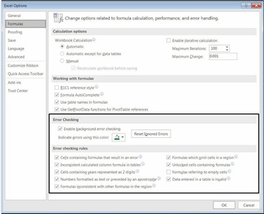 FIGURE 5-12:
The Excel Options
dialog box.
Another part of Excel’s error checking feature can be accessed via the Error Checking or Trace Error options, also in the Formula Auditing section on the Formulas tab in the Ribbon. As shown in Figure 5-13, the error checking
option will fi any Excel errors on the sheet, and then the Trace Error tool will apply Trace Precedents to fi the source of the error.
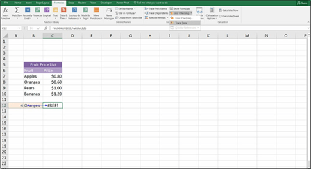 FIGURE 5-13:
The Error
Checking tool.
» Watch window: Another tool in the Formula Auditing section of the Formulas tab in the Ribbon is the Watch window. If you have output cells you’d like to keep an eye on, this tool displays the result of specifi cells in a separate
window. The Watch window is useful for testing formulas to see the impact of a change in assumptions on a separate cell or cells.
For example, in the integrated fi model you create in Chapter 12, you can add a watch to the ending cash fl As shown in Figure 5-14, select the cell you want to monitor — in this case, cell N42 on the IS Cash Flow sheet. Click the Formulas tab in the Ribbon and then select the Watch Window button in the Formula Auditing section. When the Watch Window dialog box appears, click Add Watch, as shown in Figure 5-14, and then click the Add button.


