Excel Tools and Techniques for Financial Modeling
 hen you’re using Excel for the purpose of financial modeling, much of the emphasis is on selecting the right function to include in the formu- las to calculate the results of the model. Besides functions, a number of
tools and techniques are also useful to include in your models. Chapter 7 focuses on Excel formulas. This chapter looks at some of the other practical tools and techniques commonly used in financial modeling in Excel.
 Referencing Cells
In Chapter 3, I explain why not every spreadsheet built in Excel is a financial model. In order to be able to call your spreadsheet a financial model, it must
contain formulas. And in order to build formulas, you need to reference cells. It follows therefore that as a financial modeler, you must understand how to refer- ence cells in Excel.
An Excel worksheet is made up of over a million rows and more than 16,000 columns. Each of these cells is referred to like the coordinates of a map, and the cell references are what you use to build the formula. For example, in Figure 6-1, the cost of $450 has been entered in cell B2. So, if you want to use that value in another cell, you would use the cell reference =B2.
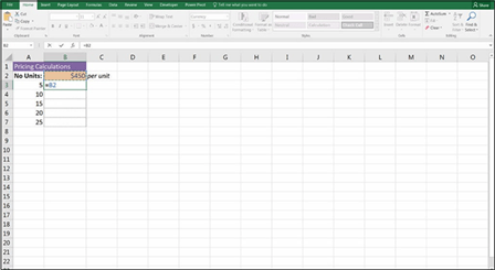 FIGURE 6-1:
Cell referencing.
 You can download File 0601.xlsx at www.dummies.com/go/financialmodeling inexcelfd.
 This kind of reference is called a relative cell reference, and it’s the default way that Excel treats the reference when you first link to a cell. There are three types of cell references, however, and the way you choose to reference a cell will depend on how you want your formula to change when you copy it to other cells:
 » Relative cell reference: Both the column letter and the row number change relative to where the formula is copied. A relative cell reference is simply a cell name, such as B2.
» Absolute cell reference: The column letter and row number of a cell name are preceded by dollar signs, such as $B$2, to indicate that the cell reference should not change when copied.
 » Mixed cell reference: Either the column letter or row number is preceded by a dollar sign to indicate which of these is to remain unchanged when copied. Both $B2 and B$2 are examples of mixed cell references.
Understanding the difference between relative, absolute, and mixed cell referenc- ing is important when it comes to efficiently building your financial models and maintaining formula consistency. Formula consistency is critical for best practice in financial modeling (and in any other sort of analysis using Excel). In order to have consistent formulas across and down the block of data, you need to under- stand how cell referencing works. Although cell referencing is a very basic feature of Excel that is taught in introductory Excel courses, it’s surprising how many modelers don’t recognize its importance.

 The dollar sign in cell referencing tells Excel how to treat your references when you copy the cell. If there is a dollar sign in front of a row number or column let- ter, the row or column does not change when you copy it. Otherwise, it does change. So an absolute reference will not change its cell reference when you copy it, whereas a relative reference will.
I walk you through each of these types of cell referencing in greater detail in the following sections.
Relative cell referencing
Relative cell referencing is the default in Excel. For example, Figure 6-2 calculates the total price by referring to values in cells B2 and A3. The asterisk is used to multiply the numbers in the two cells.
 FIGURE 6-2:
Relative cell referencing.

 Although you can manually type out a cell reference, this may introduce hard-to- detect typing errors. To avoid this problem, enter your cell reference by typing the formula up to the point of the cell reference and then select the cell with the value to be used in your formula. You can do this by clicking the cell with your mouse or using the arrow keys on your keyboard. When you select a cell, Excel automatically places the cell name in your formula.
When you copy a formula with relative references to the cell below, the row num- ber of the references adjust accordingly. In the same way, when you copy the formula to the next cell over, the column letters changes. For example, when the formula in cell B3 is copied down the range, the references automatically change, as shown in Figure 6-3, and the results will be wrong!
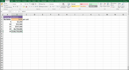 FIGURE 6-3:
A relative reference copied down (incorrect
and not recommended).
To get the correct result using relative references, you’d need to re-create the formula five times instead of copying it down, as shown in Figure 6-4.
Although this does give the correct results, it’s not the fastest and easiest way of building this formula. There are several reasons why this solution is not recommended:
 » It takes a lot longer to build.
» The formula is prone to error because you’re far more likely to accidentally pick up the wrong cell.
» Updating it will mean having to update each and every formula in the range.
» It’s more diffi for someone else to follow and, hence, more diffi to audit.
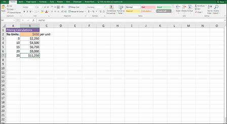 FIGURE 6-4:
A relative reference built separately (mathematically correct but not recommended).
Absolute cell referencing
A much better solution would be to use the formula =$B$2*A3 and then copy the formula down the range, as shown in Figure 6-5. Putting one dollar sign before the column letter and another before the row number in the cell reference anchors the reference when it’s copied. This is called an absolute reference.
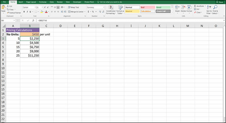 FIGURE 6-5:
An absolute reference copied down (recommended).
In this example, the $B$2 part of the formula is an absolute reference, and the A3 part of the formula is a relative reference. As shown in Figure 6-5, the absolute reference remains constant, but the relative reference changes when it’s copied down.
Let’s take a look at a practical example and apply relative and absolute cell refer- encing to a very simple financial model. You’ve been given the annual salaries for staff members who will work on a particular project. Assume that each person works 260 days in the year, and each person must work 60 days on this project. Calculate the total staff cost of the project.
Download File 0601.xlsx at www.dummies.com/go/financialmodelinginexcelfd and select the tab labeled 6-6, or open a blank workbook and enter and format the data as shown in Figure 6-6. Then follow these steps:
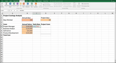 FIGURE 6-6:
Calculating daily
staff rate using
absolute referencing.
-
In cell C6, enter the formula =B6/B3.
This formula calculates the daily rate of each person by dividing his annual salary by the number of days he works per year. The formula result is $923.08.
-
Press F4 to apply absolute referencing.
The formula changes to =B6/$B$3.
-
Copy this formula down the column.
Now you need to calculate what those project costs are based on the daily rate by multiplying the number of project days by the daily rate.
- In cell D6, enter the formula =D3*C6.
-
When you copy it down, you want the project days reference to remain
constant, so press F4 to fi this reference.
The formula is =$D$3*C6 with the resulting value of $55,385.
- Copy this formula down the column.
-
In cell D10, enter the formula =SUM(D6:D9).
The result $146,769, which is the total project cost.
- Compare your results to Figure 6-7.
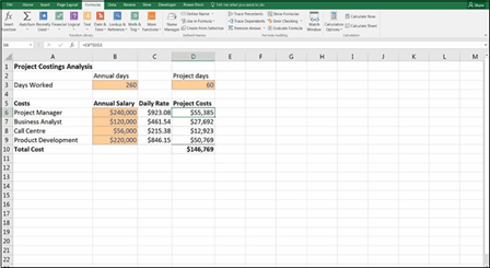 FIGURE 6-7:
Completed project costs.
You can perform some sensitivity analysis by changing the number of project days in cell D3 from 60 to 65. Change the cost for the business analyst in cell B7 from $120,000 to $150,000. Observe the eff it has on the project costs.
Mixed cell referencing
Mixed cell referencing is a combination of relative and absolute referencing; one part of the reference is absolute, and the other is relative. When you add a dollar sign before the row, the row remains anchored when the cell is copied; when you add a dollar sign before the column, the column remains anchored when the cell is copied.
For example, if you create the reference =B2 in a cell, and then copy that reference down, it will change to B3. If you add some anchoring, here are the results in each case:
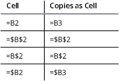
The dollar sign anchors a row number or column letter when you copy it. You can anchor both the column and the row (absolute referencing), or you can anchor one or the other (mixed referencing).
Mixed cell referencing is a concept critical to good financial modeling practice, so it’s important for a financial modeler to understand this fundamental concept. Used effectively, mixed cell references make your model
 » Faster to build and more effi
» Less prone to error
» Quicker, easier, and cheaper to audit

 The easiest way to quickly add absolute and mixed cell referencing is to press F4 immediately after adding the reference to the formula. This keyboard shortcut cycles through combinations of relative and absolute referencing. You can repeat- edly press F4 after entering the cell name in a formula to cycle through the mixed references. For example, type =B2 and then press F4 to display =$B$2. Press F4 again to display =B$2. Press F4 again to display =$B2. And press F4 again to display =B2.
Let’s look at a practical example of how to use mixed cell referencing. In the follow- ing example, you want to calculate how much you’d receive in interest under three different portfolio amounts and three different interest rates. The most effi
way to perform this calculation is to create a single formula with appropriate refer- ences and then copy that formula to other cells. You need to create a formula that multiplies the interest amount in row 1 and the borrowing amount in column A.

 Instead of creating nine different formulas, you’re creating only one single formula using mixed cell referencing, which you can then copy across, saving you time and reducing the possibility of error.
Follow these steps:
- Download File 0601.xlsx from www.dummies.com/go/financialmodeling inexcelfd
and select the tab labeled 6-8 or create a blank workbook and enter and format the data as shown in Figure 6-8.
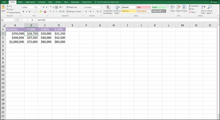 FIGURE 6-8:
Mixed cell referencing.
- In cell B2, type = and then select cell A2 by clicking it or pressing the arrow key.
- Press F4 three times to display the mixed reference $A2.
-
 Type *, select cell B1, and this time press F4 twice to display the mixed reference B$1.
To anchor the row, put the dollar sign before the row. To anchor the column, put the dollar sign before the column.
-
 Press Enter to show the formula =$A2*B$1 in cell B2.
The result is $18,750 as shown in Figure 6-8.
- Select cell B2 and copy it across and down the rest of the block of data.
Copying and pasting can be done in a several diff ways. Choose the
option that suits you best:
-
Go to the lower-right corner of cell B2 and select the fi handle with the
mouse. Drag it across to cell D2 and release the mouse. Then drag down
to row 4.
-
-
Copy cell B2 with the shortcut Ctrl+C, and select the entire block either with the mouse or by holding down the Shift key together with the right arrow
and down arrow. Press Enter to paste.
-
Highlight the entire block of data either with the mouse or by holding down the Shift key together with the right arrow and down arrow. Use the
shortcuts Ctrl+R and Ctrl+D to copy right and copy down.
-
Review the results.
Note how your carefully crafted formula generates data for the entire block of
cells. Compare your worksheet to the one shown in Figure 6-8.

 Maintaining consistency of formulas is a fundamental technique of financial modeling that will save you and anyone else using your model a lot of unnecessary time in building, checking, and auditing the calculations.
When formulas make calculations based on data stored in your spreadsheet, use cell references wherever possible, instead of typing the actual data. Typing num- bers into formulas is called hard coding, and it should be avoided unless the num- bers are source data — and, if so, documented as such. This rule is also important to follow when building your model because it makes your models much easier to update, both for you and others using your model. If you’ve used cell references instead of hard-coded the numbers into the formula, and you change a value in a cell referenced by a formula, the formula automatically recalculates.
.


