Rounding with MROUND
In the previous-edition of this book, we introduced the ROUND, ROUNDUP, and ROUNDDOWN functions. When we use the increase and decrease decimal icons in Excel, we are formatting a cosmetic change to values by rounding them. This does not change the underlying raw data value in the cell.
To apply rounding to a value to use in calculations, we need to round by using a formula. We will now increase our knowledge by extending it to include the MROUND function. As a recap, the ROUND function allows us to round a number to a specific number of digits (decimal places). The MROUND function rounds numbers to the nearest multiple.
Note that the MROUND function will affect the result of formulas as it modifies cell data. Let’s run through an example, as follows:
- Open the SSGPetFormat.xlsx workbook to follow along.
- Before we begin, let’s insert a new column in between the Amount Owing column and the existing Total Owing: Medicines column.
- As an introduction to the MROUND function, we will round the values in the Amount Owing column. The result of the formula will be in cell N2, as illustrated in the following screenshot:
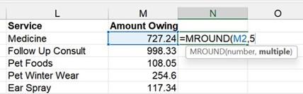
Figure 12.13 – MROUND function to the nearest 5
- Type =MROUND( then click on the value in M2. Add a comma to separate the arguments, then indicate the multiple types you require. For this example, we will round to the nearest 5.
- Press Enter to confirm. You will see the following result:
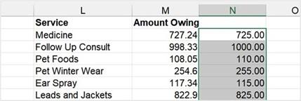
Figure 12.14 – MROUND function result
- Notice the difference between the values in the two columns.
The FLOOR function is like the MROUND function, although it rounds down to the nearest multiple of significance to zero. Let’s look at a practical example of this in the next section.
Rounding with the FLOOR function
Here, we will look at another method to round values. This time, we are rounding the nearest significant value to zero. Proceed as follows:
- Continuing with the same workbook, click into cell O2.
- Start to type the function, as follows: =FLOOR(.
- Click on cell M2 as per the previous example, then add a comma.
- For this example, we will also use 5 to locate the nearest multiple of 5 to 0.
- Press Enter to see the result in cell O2. Copy the formula down the column, as illustrated in the following screenshot:
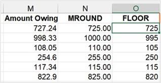
Figure 12.15 – Difference between MROUND and FLOOR
- Notice the difference between MROUND and FLOOR in column N and column O. The opposite of the FLOOR function is the CEILING function.
- Add another column in the worksheet so that we can explore this. Click into cell P2
to start the function.
- Type =CEILING(M2,5) to find the closest multiple of 5. Press Enter to see the result. It should look like this:
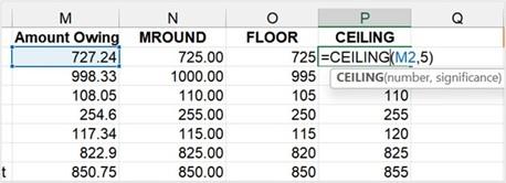
Figure 12.16 – CEILING function
There are many methods for rounding values on a worksheet, and this section contains just a few of these methods. The next section will focus on the TRUNC function.
Returning integers
The INT and TRUNC functions have one similarity: they both return integers. INT rounds down to the nearest integer, basing it on the fractional part of a number, while TRUNC removes the fractional part of the number and truncates it to an integer. In layman’s terms, it removes decimal places.
We will not go through this function step by step as the syntax is very similar to that shown in the previous sections. The following screenshot details the function and the result to display one decimal place only:
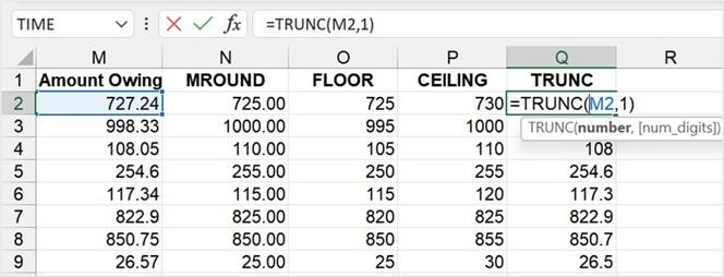
Figure 12.17 – TRUNC function
Remember that any of these functions can be added to existing formulas to gain the result you require.
The next section concentrates on a function that enables a wide selection of mathematical functions within it to customize the output. The function is quite new, so if constructed in versions earlier than Excel 2010, the output will return a #NAME! error.
Working out how to use AGGREGATE
The AGGREGATE function is a useful tool to obtain, for instance, the maximum values in a range without including any error values in the selected range. The function can be constructed to ignore hidden rows and errors. It consists of required arguments from which you can choose further functions to base your result.
The syntax for the AGGREGATE function looks like this: =AGGREGATE(function_ num, options, array, [k]).
The following table explains the relevant syntax arguments:
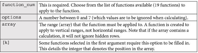
Table 12.2 – AGGREGATE syntax
Although there are instances where we can use basic formulas to reach a result instead of the AGGREGATE function, this might not be as fluid as we need.
For instance, when we construct the AVERAGE function, the following constraints could impact the result:
- Any hidden column data is included in the result.
- Includes cells containing 0s in the formula result.
- Ignores logical values.
- Ignores numbers entered as text .
These constraints could return an incorrect result that could impact other formulas in the workbook.
The AGGREGRATE function arguments, although a bit of extra work for the end user, allow further customizations utilizing 19 functions with 8 options to choose from.
Let’s work through an example, as follows:
-
Open the Training Schedule.xlsx workbook. Make sure you are on the
Overtime worksheet.
- The worksheet is set up to display overtime for trainers for remote training sessions per offi . We will work out the sum of overtime per trainer in cell B13 as an example.
- Start the formula by typing this into cell B13: =AGGREGATE(. You can see an illustration of this in the following screenshot:
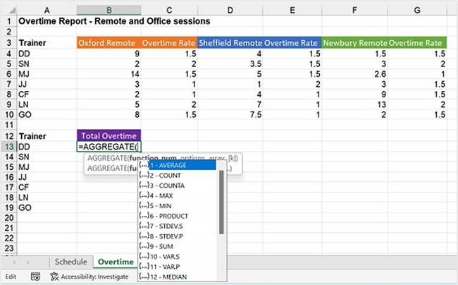
Figure 12.18 – AGGREGATE function syntax
- A drop-down list will appear straightaway that houses 19 different functions to choose from. Double-click to select the SUM function from the list.
- Insert a comma, after which the next argument will appear, displaying the eight options to choose from, as illustrated in the following screenshot:
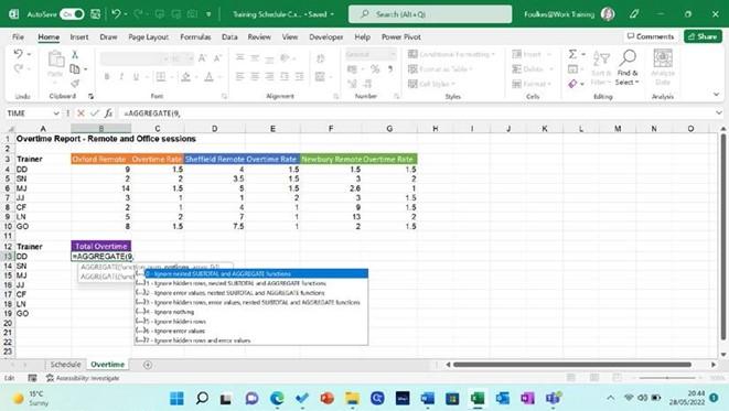
Figure 12.19 – Argument options
-
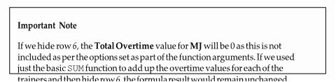
This is the step where you could be more concise to refine the result of the formula so that calculations work effectively against your dataset. For this example, we will double-click option 5, as we may hide rows at some point as the dataset grows over time. This ensures that the formula will not include values from any hidden rows in the worksheet.
- Insert a comma to move to the next argument and select a range (array) in the worksheet. Select cells B4, D4, and F4, as illustrated in the following screenshot:
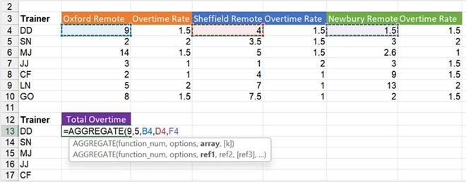
Figure 12.20 – Array argument
- Lastly, press Enter to see the result in cell B13. Copy the result to the rest of the column to see the result of total overtime for each trainer.
- This function is a powerful function and something to consider as an alternative when using basic functions such as SUM and AVERAGE.
Just to mention here that the SUBTOTAL function is also part of the Math & Trig
functions. The syntax is like that of the AGGREGATE function.
The AGGREGATE function is the most updated function with more option arguments than its predecessor, SUBTOTAL. The main difference between these functions is that with SUBTOTAL, we can choose to include or exclude manually hidden rows.
The next section concentrates on an engineering function. Although not directly part of the
Math & Trig library, it is relevant and worth mentioning. Let’s learn a little about this now.