Converting the month name to a month number
To convert the month name to a month number, proceed as follows:
- To return the month name to a month number, we simply use a combination of functions—namely, =MONTH(DATEVALUE(J2 & “1”)); & “1” is necessary for the DATEVALUE function to comprehend that it is a date.
- Try this out in cell K2 of the EXAMPLES worksheet (Date and Time.xlsx) workbook, as illustrated in the following screenshot:
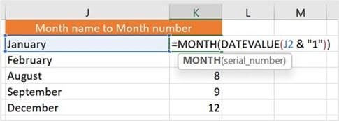
Figure 11.12 – Converting the month name to the month number
-
The names of the months have been converted to the month number in K2.
The following topic will explain how to quickly calculate a future date based on the number of days from the current date.
Working out the future date from the days specified
The WORKDAY function returns the date for a specified number of working days entered from a specific date.
Make sure you are on the EXAMPLES worksheet of the Date and Time.xlsx workbook. In cell A16, we have the Start Date of Project value, and in B16, we have listed the number of days till the end date of the project. We would like to find out the project end date. Here’s how we do this:
- In cell C16, start the formula by entering =WORKDAY(.
- Click on the Start Date of Project cell (A16) then add a comma, and finally, add the number of working days. For the following example, we are using a cell reference that contains the number of working days in cell B16:
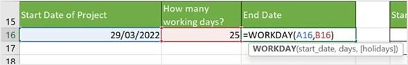
Figure 11.13 – Working out the date from a specified number of days
- Press the Enter key to see the End Date value in cell C16.
We can extend this function to add any holidays during the working day period specified, as follows:
-
In cells G16 and G17, we have entered two holiday dates we would like to include in the formula so that it works out the correct number of working days, taking holidays into account. Enter the formula as follows: =WORKDAY(E16,F16,G16:G17). You can see an illustration of this in the following screenshot:
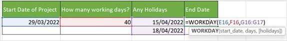
Figure 11.14 – Using the WORKDAY function to add holidays
- Press Enter to see the Project End Date value.
Experiment with these functions and combine them to get the result you desire.
Finding the last day of a month after adding specified months
It is useful to find out the last day of a month from the starting month after adding a specified number of months. Let’s investigate the EOMONTH function, as follows:
-
In cell J16 in the following screenshot, we have entered a Start Date value. In K16, you will see the number of months we will add to the existing start date. Let’s build a formula in cell L16 to calculate the last day of the month, taking into account the number of months entered in K16:
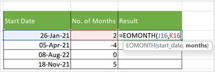
Figure 11.15 – Working out the last day of the month
- Enter =EOMONTH( in L16. Click J16 to select the start date (26-Jan-21), then add a comma to separate the arguments.
- Click on cell L16 to take into consideration the months entered in the cell.
-
Press Enter to see the result in cell L16. Note that the result is formatted as a serial number. To format as a date, use the relevant Number Format dropdown to select Short Date.
- The date displayed in L16 is the last day of the month, 2 months from January 26, 2021.
- Autofill the formula to the rest of the cells to fill in the relevant dates for each of the start dates.
The next couple of topics are for those interested in calculating the age of an employee or working out the date employees will retire.
Calculating the current age from a birth date
There are two common types of functions that calculate the age from a specified date. Let’s investigate these in the next topics. Both the functions covered here are functions that every human resources (HR) employee should know.
Using the YEARFRAC function
The YEARFRAC function is used to calculate the accurate age of—for instance—an employee from their given birth date. Here’s how you can use this:
- Using the same workbook as prior topics, Date and Time.xlsx, we will click on the EMPLOYEES worksheet.
- The worksheet contains employee information for the Safest Solutions theme park. Employee start dates are evident in column I, and birth dates in column G. Firstly, we would like to find out the employee’s age in years in column H.
-
Click into cell H5 to construct the formula. We will be using the YEARFRAC
function for this example. The YEARFRAC function syntax is shown here:
=YEARFRAC(start_date,end_date,[basis]).
- Type =YEARFRAC(, then click on G5 as this is our start_date value (birth date). Add a comma to separate the arguments, then type TODAY() as the end_date value as we are working out how old the employee is today.
- End the formula off with another ) to close the arguments and finish the formula. You can see the formula in the following screenshot:
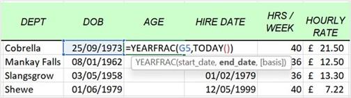
Figure 11.16 – YEARFRAC function to work out the age of employees
-
Press Enter to see the age of the first employee. If a date is presented in the answer cell, be sure to change the Number Format value to General so that it displays the age correctly. Autofill to the rest of the column.
- If you would like to round down to the nearest integer, add the INT function at the start of the formula, as follows: =INT(YEARFRAC(G5,TODAY())). Remember to add an extra ) at the end of the formula to include the function as you have three function arguments in your formula.
We can also use the YEARFRAC function to determine the age of an employee at a specific future date. Here’s how we’d go about this:
- We will continue with the previous worksheet to work out the future age in cell I5 based on a specific date in cell I3—namely, 31/12/2025.
- In cell I5, enter the following formula: =YEARFRAC(H5,$I$3).
- Make sure cell I3 is referenced as absolute so that the reference does not move down when using the autofill to copy the formula to the rest of the cells.
- Press Enter to see the age of the employee on 31/12/2025. Copy down to the rest of the cells.
Let’s look at the DATEDIF function in the following section.
Using the DATEDIF function
DATEDIF is a function that works out the age of the employee to display the year, month, and day in the cell. When working with the DATEDIF function, we will need to type the function into the cell to construct it from scratch. The DATEDIF function is not resident in the drop-down list of functions in Excel, and neither is the tooltip to guide you when constructing arguments. We will need to remember the function and construction arguments. Proceed as follows:
- Using the same workbook as prior topics, Date and Time.xlsx, make sure you are on the EMPLOYEES worksheet.
-
Employee age is calculated in years in column H. If we wanted to work out the year, month, or day instead, we could need to use a different function. Let’s calculate this in column J of the worksheet.
-
Click on cell J5 to construct the formula. We will be using the DATEDIF
function for this example. The DATEDIF function syntax is shown here:
=DATEDIF(start_date,end_date,unit). We will build this formula using different units to achieve the result.
-
Type =DATEDIF( then click on G5 as this is our start_date value (birth date). Add a comma to separate the arguments, then type TODAY() as the end_date value as we are working out how old the employee is today. Add a comma again to specify the last part of the formula.
To find out more about the DATEDIF function, click on the blue DATEDIF link in the syntax, as shown here:
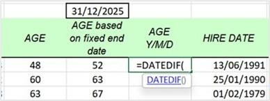
Figure 11.17 – The DATEDIF function
- The first unit we require is the year, so we need to enter Y in the formula as the unit. Close the function bracket by adding ).
-
As we would like to see the word years after the year unit, we need to include
” years ” after the function to expand the text string. Press the spacebar, then add another &.
- Copy the first DATEDIF function and amend the unit to reflect “YM”.
-
Add & to expand on the formula, followed by the spacebar, then include
” months ” after the function to expand the text string. Your formula should look exactly like this: =DATEDIF(G5,TODAY(),”Y”)&” years “
&DATEDIF(G5,TODAY(),”YM”)& ” months”. You can see this displayed in the following screenshot:
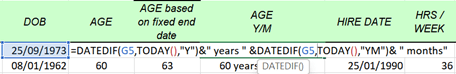
Figure 11.18 – Formula to work out the age of employees
- Press Enter to see the result and copy it down to the rest of the employees, as illustrated here:
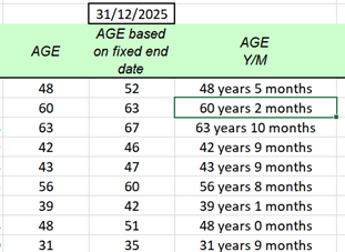
Figure 11.19 – Employee age in years and months
You have now learned to apply the YEARFRAC and DATEDIF functions. In the next section, we will look at how to calculate retirement dates and the remaining retirement years for employees.