Evaluating array formulas
We can evaluate part of an array by selecting the part of the array formula and then pressing F9 on the keyboard to show values. This is a great way of checking whether the array is using the correct cells:
- Select the array cells to evaluate.
- In the formula bar, select the part of the array formula to investigate.

Figure 10.6 – Selecting the part of the array to evaluate
- Press F9 on the keyboard to display the values. Note that if you do not select part of the formula prior to pressing F9, the formula will update to the calculated value only.

Figure 10.7 – Pressing F9 to evaluate the formula
- Press Esc on the keyboard when complete.
Now that we are confident in terms of how to create and edit arrays, we will learn more about the new array formulas in the following topic.
Investigating new functions
Excel 2021 has a few new functions, namely, XLOOKUP, LET, XMATCH, and a couple of dynamic Array functions. We will discover these in the following topics.
New dynamic array functions
In the previous chapter, we introduced the FILTER and UNIQUE functions. The FILTER function is part of the new dynamic array formulas in Excel 2021. When we apply this function, the results spill from a single cell into the adjacent cells. Normally, when using the traditional filter in Excel, it will not update as new data is entered into the workbook – you would have to recalculate or update the results.
Dynamic arrays are perfect since, when the underlying data (source data) is updated, all lists based on that dataset are updated automatically.
Along with the new FILTER function, we also have a couple of other functions added to the list of dynamic array formulas, namely, SORT, SORTBY, UNIQUE, SEQUENCE, and RANDARRAY.
Let’s recap the FILTER function and combine it with the CHOOSE function to extract the cases sold of a particular wine label above 300:
- Open the workbook named MattWinery.xlsx.
- On the first sheet, we have a dataset relating to wines and the number of cases sold per region. The dataset contains column headings in Row 1.
- We would like to set up a filter to split the regions and cases sold above 300, per label selected in cell K2, into columns M and N, respectively.
- As we require the headings Region and Cases Sold for the output columns, we need to copy the existing headings and paste them into cells M1 and M2.
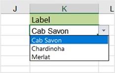
- In cell K1, enter the heading Label and create a validation rule to list the following items in cell K2: Cab Savon, Chardinoha, and Merlat.

Figure 10.8 – Validation rule to define the Label categories
- In cell M2, construct the following formula using the CHOOSE and FILTER functions: =FILTER(CHOOSE({1,2},Table1[Region],Table1[Cases Sold]),Table1[Label]=K2)

Figure 10.9 – The FILTER and CHOOSE functions in cell M2
- The result will spill into columns M and N accordingly, based on the selection in cell K2. Choose another label type from the validation rule in cell K2 to see the table update.
Let’s now look at another two new dynamic array functions.
The SEQUENCE function generates a list of sequential values. We can use this function to create codes or for a specific range of values:
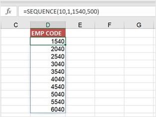
- Click on Sheet 2. In cell D1, enter the heading EMP CODE. In cell D2, enter the following formula: =SEQUENCE(10,1,1540,500).
- Press Enter to populate the list. To clarify the formula syntax, the number 10 refers to the number of rows to fill, 1 means a single column, 1540 refers to the start number, and 500 the increments between each.

Figure 10.10 – Sequence function in cell D2
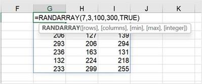
The RANDARRAY function returns a list of values across rows or columns. You can generate a list of accidental whole numbers according to a given constraint, decimal numbers according to a given constraint, or a set of accidental values. This new function is a replacement for the former RAND and RANDBETWEEN functions.

Figure 10.11 – The new RANDARRAY function syntax
In the previous edition of our book, Learn Microsoft Office 2019, we explored the application of conditional logic in a formula using IF, AND, and OR. We will briefly recap the IF function with a few more examples to enhance what we have learned.


