Home » Civil Engineering Projects » Date-Time Functions and Enhancing PivotTable Dashboards

Civil Engineering Projects

Date-Time Functions and Enhancing PivotTable Dashboards

learn

February 5, 2023

17 Views 0

SaveSavedRemoved 0

Date-Time Functions and Enhancing PivotTable Dashboards

In this chapter, we will explore date functions and look at how to work with time. Here, we concentrate on DATEDIF(), YEARFRAC(), EDATE(), WORKDAY(), and many more functions to be more productive in the workplace. In addition, a large part of this chapter will explore a host of PivotTable customizations and a walk-through on creating dashboards. We will also learn to construct the GETPIVOTDATA function to reference cells in a PivotTable report.

The following topics are covered in this chapter:

• Working with dates
• Working with time
• Enhancing PivotTables
• Creating dashboards
• Additional PivotTable customizations

Technical requirements

Before starting this chapter, you should have adequate file management skills to be able to save workbooks and interact with the Excel 2021 environment comfortably. We assume that you are also able to construct a formula and manage worksheet data. The examples used in this chapter can be accessed from https://github.com/ PacktPublishing/Learn-Microsoft-Office-2021-Second-Edition.

Working with dates

In this topic, we will enhance our knowledge of date functions within Excel 2021.

Understanding how dates are interpreted

After typing a date into a worksheet cell, we will only see the formatting of that date (the cosmetic change). If Excel recognizes the date you have typed into a cell on the worksheet, it will automatically align the date to the right of the cell immediately, and apply the date format. To understand visually how a date is actually presented in the cell behind the formatting, we could remove the cell formatting. Let’s look at an example.

If we type the number 1 into a cell and then format the cell to display the Short Date format, we will visually see the number 1 displayed as the date 01/01/1901 in the cell. 01/01/1901 is the actual starting date in Excel, and 31/12/9999 is the end, or last date, that Excel interprets. When we remove the formatting, by clearing the format (Home | Clear

| Clear Formats), we will see the actual whole number behind the cosmetic format. Note that we can also use the General number format to display the raw date in the cell. Excel works and stores dates as serial numbers in the background. The following screenshot provides a representation of cosmetic and raw date functions:

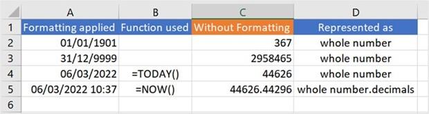
Figure 11.1 – Representation of cosmetic and raw date functions

The date and time in cell A5 are represented as a whole number for the date portion of the function, and the decimals represent the time portion, as seen in cell C5 (raw data, without formatting applied).

If we wanted to display a date as text in a column, we would simply apply the Text format to the column that would align the data to the left of the cell, indicating that the data is not represented as a date. We could also indicate this using an ‘ (apostrophe) before entering a date into a cell to force it to the Text format in the cell, as illustrated in the following screenshot. The apostrophe is a silent character and will not show in the cell once you have pressed Enter:

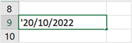
Figure 11.2 – Forcing a date to be displayed as text in a cell

We can use arithmetic to add and subtract days from dates easily or use various Excel functions in order to do so. So, to add a day to the date in cell A4 (06/03/2022), we would simply type + 1, or -1 to subtract a day from the date.

In the following section, we will learn all about how to construct date functions and become knowledgeable about when to apply different date functions in Excel.

Exploring date functions

In our previous book, Learn Microsoft Office 2019, we learned about the =TODAY() and =DAY() functions. Throughout this chapter, we will use the type method to access different date and time functions. Don’t forget that we can also access all the date and time functions, along with their explanations, by visiting Formulas | Date & Time, as illustrated in the following screenshot:

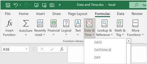
Figure 11.3 – Date & Time drop-down list, located on the Formulas tab

In the following table, we define a couple of date functions, some of which we will explore in further sections.

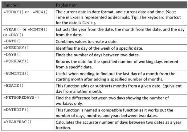
Table 11.1 – Date functions

When working with dates, always make sure that any dates imported into Excel are formatted correctly, and that cells are aligned correctly. #NUM! or #VALUE! errors can appear when this is the case.

Extracting the day, month, or year

We can extract various elements (day, month, or year) from a date into separate cells on the worksheet using the relevant function. There are many different scenarios in which you may want to achieve and extract the elements from a date—for instance, you are only interested in the year of a vehicle or may visually just need to filter the year in a separate column. As is the case with many features of Excel, there is always more than one method to achieve something, or the method could be dependent on a specific outcome you require. To extract an element from a date, proceed as follows:

• Open the workbook named Date and Time.xlsx. Navigate to the
  

  EXTRACT worksheet.
  

• On this worksheet, there is an existing DATE of HIRE column that includes the date of hire for each employee.
• We will separate the day, month, and year from the existing date in cell G5 and place these in the respective columns on the worksheet (H5, I5, J5). We will use the following function syntax in order to do so: =DAY(Serial_Number) or

  =MONTH(Serial_Number) or =YEAR(Serial_Number).
  

• Click on cell H5, then construct the formula by pressing =DAY(.
• Click on cell G5 to extract the day from the cell. Press Enter to confirm and display the day in cell H5. Do the same for the month and year cells, replacing the DAY function with either the MONTH or the YEAR function when constructing the formula. The process is illustrated in the following screenshot:

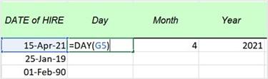
Figure 11.4 – The DAY function in action

• Select cells H5:J5, and use the AutoFill handle to copy the formula to the rest of the employees on the worksheet.

Formatting dates as values

To format dates as values, proceed as follows:

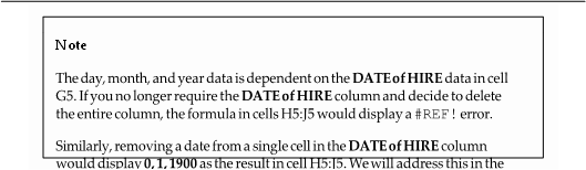
• Following on from the previous example, we would now like to remove the DATE of HIRE column from the worksheet. As explained in the Note information box, we would return #REF! errors in the cells if we removed the entire column. Prior to doing so, we can format the dates to values so that they are static in the cell and not dependent on any formula.
• Make sure you are on the EXTRACT worksheet (Date and Time.xlsx).
  
• Select the cell range H5:J98.
• Hover your mouse pointer, without clicking, to the outside border of the selected range.
• Right-click, then hold down the mouse pointer and drag the range slightly off its placement cells, then back in position again.
• You should now see a shortcut menu appear with several options to choose from.
• Click to select Copy Here as Values Only, as illustrated in the following screenshot:
  

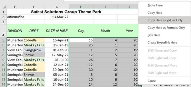
Figure 11.5 – Copy Here as Values Only

• Delete the DATE of HIRE column.
  
• The values remain in cells H5:J5 and are not affected by the deletion of the source column anymore.

We separated the contents of a single cell into three cells to display the day, month, and year independently of each other. How would we combine separate values to form a date in a single cell? Let’s try the opposite now in the following topic.

Formulating a date from worksheet cells

We currently have the date, month, and year values in separate cells on the EXTRACT

worksheet. Follow the next steps to combine them:

• Make sure you have selected the COMBINE worksheet in the Date and Time. xlsx workbook.
  
• Click into cell G5 as this is the cell in which we would like to construct our formula to pull through the day, month, and year values from the EXTRACT worksheet. We will use the DATE function. The DATE function syntax is

  =DAY(year,month,day).
  

• Type =DAY( in the cell, then navigate to the EXTRACT worksheet.
  
• Click on the Year value first in cell I5 followed by a comma, click on cell H5 followed by a comma, then—finally—click on cell G5, as illustrated in the following screenshot:

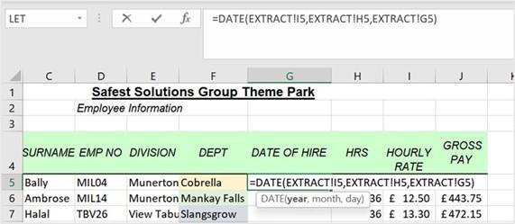
Figure 11.6 – The DATE function collecting the year, month, and date from another worksheet

• Press Enter to see the result. Notice how the formula has referenced the different worksheets used to collect the year, month, and date.

• Fill the contents of the cell down so that all dates are pulled through for each employee. Please note that any changes on the EXTRACT worksheet will amend the dates on the COMBINE worksheet unless you format these as values.

Now that you have learned to break dates apart and put them back together again, let’s look at how to subtract or add months from a given date.

Subtracting months from a date

We can subtract or add months from a date to find out a future or past date. The EDATE function is perfect for projecting a payment due date for a term of purchase, or payment due date on a certain length of membership, or for finding out when the membership started by subtracting the length of the membership term. Here’s how you can use this:

• Make sure you are on the EXAMPLES worksheet in the Date and Time.xlsx
  

  workbook.

• Firstly, we will work out the New Date value by subtracting the number of months in cell F3 from the Date value in cell E3. Once complete, we will autofill the results to row 4. The function we will use is EDATE. The EDATE syntax is

  =EDATE(start_date,months).
  

• Click into cell G3, then start the formula by typing the =EDATE( function.
  
• Click to select cell E3, the start_date value, press the comma to separate the arguments, then add the subtract operator and click on cell F3, which contains the number of months to subtract. The process is illustrated in the following screenshot:

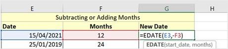
Figure 11.7 – Subtracting months from dates

• Press Enter to see the New Date value.
  
• If the cell is not formatted to a date format, the serial number will be displayed in the cell. Format the relevant date format to correct it. Autofill the formula result to cell G
• Let’s work out the second example by adding 6 months to the payment date to project the Last Payment Due date.

• Click on cell F6, then type the =EDATE( formula, as illustrated in the following screenshot:

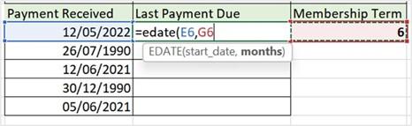
Figure 11.8 – Adding months to dates

• Click on cell E6, and add a comma to separate the arguments.
• Click on select cell G6, which contains the Membership Term value. Note that we can type the value into the formula construction instead of using a cell reference, but if we want to change the Membership Term value at any time, we would want the formula to update automatically.
• Press Enter to see the result, then autofill to the range F7:F10. If the Membership Term value changes, simply enter the new term value into cell G6 to update the values.
• Now, let’s see how we would add half a day to a particular date.

Adding half a day to a date

To add a day to a date, we would simply include + 1 in the formula. As we are working out for half a day, we would use 0.5. Here’s how we’ll do this:

• In cell A10 of the EXAMPLES worksheet, we have entered the =NOW function to insert the current date and time.
• In cell B10, we would like to work out the current date and time including half a day. Type the formula =A10+0.5 into B10 to find the answer, as illustrated in the following screenshot:

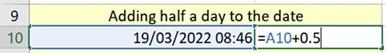
Figure 11.9 – Adding half a day to a date

• Press Enter to see the future date/time.

At times, you may need to see the actual day name in a cell, alongside a full date. This helps with closing dates for property transactions, for example. We will learn how to pull the day from the date next.

Displaying the date day

We will now learn how to convert a short date to display the corresponding day in a column, as follows:

• Open the workbook named Date and Time.xlsx.
  
• Click to access the DAY worksheet. Column B consists of property dates. In column A (Day), we would like to automatically return the day, once the date is entered in column B (Property Date).
• Select cell A2, then enter the formula =DAY(B2), as illustrated in the following screenshot. Press Enter to see the result:

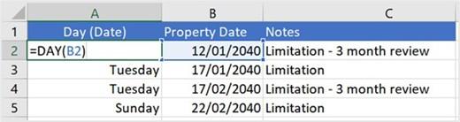
Figure 11.10 – Converting the date to the name of the day

• Notice that the result is not displaying the weekday name, only the day number. We will need to alter the format of the cell. Select cell A2 again, then visit Format Cells. Choose Custom to set the correct format. In the Type: field, enter dddd to display the date day. Look at the Sample box to see the format. The process is illustrated in the following screenshot:

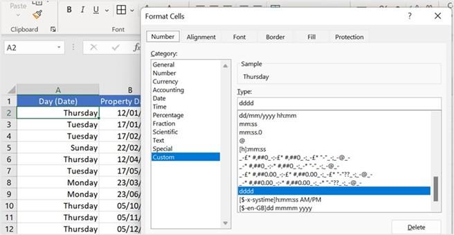
Figure 11.11 – Changing the custom format to reflect the day name

• Click OK to confirm and display the name of the day in the cell.
• Autofill the formula to cell A19. If you need to extend the selection from A2 all the way to A1048576 (the last cell in column A on the worksheet) as the worksheet data will grow over time, press Ctrl, Shift, and the down arrow.
• Every time you enter text into column B, it will automatically convert the date to the

  Day value in column A.
  

• If users edit the formula by mistake or enter in dates, and so on, simply drag the formula down again to correct it. You may prefer to lock the cells in column A so that the users cannot amend the day names. Use the =MONTH( function, then add mmmm as the Custom Format value.

If we have the name of a month in a cell and need to convert it to display the month number instead, we can use a combination of the MONTH and DATEVALUE functions. Follow the steps in the next example to explore this.

Converting the month name to a month number

To convert the month name to a month number, proceed as follows:

• To return the month name to a month number, we simply use a combination of functions—namely, =MONTH(DATEVALUE(J2 & “1”)); & “1” is necessary for the DATEVALUE function to comprehend that it is a date.
  
• Try this out in cell K2 of the EXAMPLES worksheet (Date and Time.xlsx) workbook, as illustrated in the following screenshot:
  

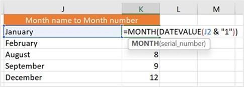
Figure 11.12 – Converting the month name to the month number

• The names of the months have been converted to the month number in K2.

  The following topic will explain how to quickly calculate a future date based on the number of days from the current date.

Working out the future date from the days specified

The WORKDAY function returns the date for a specified number of working days entered from a specific date.

Make sure you are on the EXAMPLES worksheet of the Date and Time.xlsx workbook. In cell A16, we have the Start Date of Project value, and in B16, we have listed the number of days till the end date of the project. We would like to find out the project end date. Here’s how we do this:

• In cell C16, start the formula by entering =WORKDAY(.
• Click on the Start Date of Project cell (A16) then add a comma, and finally, add the number of working days. For the following example, we are using a cell reference that contains the number of working days in cell B16:

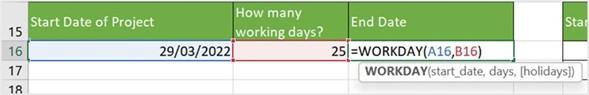
Figure 11.13 – Working out the date from a specified number of days

• Press the Enter key to see the End Date value in cell C16.
  

We can extend this function to add any holidays during the working day period specified, as follows:

• In cells G16 and G17, we have entered two holiday dates we would like to include in the formula so that it works out the correct number of working days, taking holidays into account. Enter the formula as follows: =WORKDAY(E16,F16,G16:G17). You can see an illustration of this in the following screenshot:

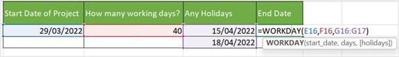
Figure 11.14 – Using the WORKDAY function to add holidays

• Press Enter to see the Project End Date value.
  

Experiment with these functions and combine them to get the result you desire.

Finding the last day of a month after adding specified months

It is useful to find out the last day of a month from the starting month after adding a specified number of months. Let’s investigate the EOMONTH function, as follows:

• In cell J16 in the following screenshot, we have entered a Start Date value. In K16, you will see the number of months we will add to the existing start date. Let’s build a formula in cell L16 to calculate the last day of the month, taking into account the number of months entered in K16:

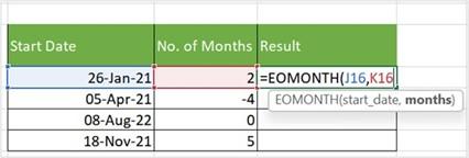
Figure 11.15 – Working out the last day of the month

• Enter =EOMONTH( in L16. Click J16 to select the start date (26-Jan-21), then add a comma to separate the arguments.
• Click on cell L16 to take into consideration the months entered in the cell.
• Press Enter to see the result in cell L16. Note that the result is formatted as a serial number. To format as a date, use the relevant Number Format dropdown to select Short Date.
• The date displayed in L16 is the last day of the month, 2 months from January 26, 2021.
• Autofill the formula to the rest of the cells to fill in the relevant dates for each of the start dates.

The next couple of topics are for those interested in calculating the age of an employee or working out the date employees will retire.

Calculating the current age from a birth date

There are two common types of functions that calculate the age from a specified date. Let’s investigate these in the next topics. Both the functions covered here are functions that every human resources (HR) employee should know.

Using the YEARFRAC function

The YEARFRAC function is used to calculate the accurate age of—for instance—an employee from their given birth date. Here’s how you can use this:

• Using the same workbook as prior topics, Date and Time.xlsx, we will click on the EMPLOYEES worksheet.
  
• The worksheet contains employee information for the Safest Solutions theme park. Employee start dates are evident in column I, and birth dates in column G. Firstly, we would like to find out the employee’s age in years in column H.
• Click into cell H5 to construct the formula. We will be using the YEARFRAC
  

  function for this example. The YEARFRAC function syntax is shown here:

  =YEARFRAC(start_date,end_date,[basis]).
  

• Type =YEARFRAC(, then click on G5 as this is our start_date value (birth date). Add a comma to separate the arguments, then type TODAY() as the end_date value as we are working out how old the employee is today.
  
• End the formula off with another ) to close the arguments and finish the formula. You can see the formula in the following screenshot:

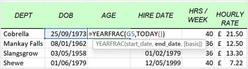
Figure 11.16 – YEARFRAC function to work out the age of employees

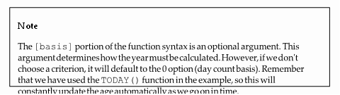
• Press Enter to see the age of the first employee. If a date is presented in the answer cell, be sure to change the Number Format value to General so that it displays the age correctly. Autofill to the rest of the column.
• If you would like to round down to the nearest integer, add the INT function at the start of the formula, as follows: =INT(YEARFRAC(G5,TODAY())). Remember to add an extra ) at the end of the formula to include the function as you have three function arguments in your formula.

We can also use the YEARFRAC function to determine the age of an employee at a specific future date. Here’s how we’d go about this:

• We will continue with the previous worksheet to work out the future age in cell I5 based on a specific date in cell I3—namely, 31/12/2025.
• In cell I5, enter the following formula: =YEARFRAC(H5,$I$3).
  
• Make sure cell I3 is referenced as absolute so that the reference does not move down when using the autofill to copy the formula to the rest of the cells.
• Press Enter to see the age of the employee on 31/12/2025. Copy down to the rest of the cells.

Let’s look at the DATEDIF function in the following section.