Filtering using Advanced Filter
In the previous edition of this book, we learned how to set up and manage sorts and filters.
Filtering data in Excel allows you to locate data very quickly, as well as eliminating certain choices (text, dates, or values) from a list’s results, or specifying categories of data to get the result you need. Filters can also be used to search if you specify the format (color) of a cell.
Instead of filtering a list with updates that are occurring in the same location, we can extract data to a different location using criteria.
Now, let’s learn how to filter using Advanced Filter.
Defining criteria
- Open the SSGAdvFilter.xlsx workbook. Our workbook contains data for a theme park.
-
To define the criteria for our filter, we need to specify a separate area on the worksheet. When we add criteria, we can indicate whether the result will be an AND or an OR criteria. For example, we can choose all the Mankay Falls employees (from the Munerton division) AND their gross pay greater than £300.
Alternatively, we can choose all the Mankay Falls (Munerton) employees with a gross pay greater than £300 OR the Cobrella (Munerton) employees with a gross pay less than £300:
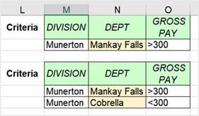
Figure 9.18 – AND/OR criteria for Advanced Filter
- Before we get started, it is important to note that the criteria must be the same as the source headings on the worksheet in terms of formatting and spelling. The best way to ensure that this happens is to copy and paste the headings you require for the criteria from the existing worksheet headings into the criteria area on the worksheet.
- Follow the example as per the previous screenshot to add the relevant criteria to the worksheet. Note that you do not have to place the criteria data on the same worksheet.
- Now that we have the criteria in place, we can create the filter and return the result.
Applying Advanced Filter
- If the result of the filter must be generated on a separate worksheet, make sure that you click the relevant worksheet before accessing the command from the ribbon. For our example, we want the result to appear on a separate worksheet. Click to create a new worksheet and name it Result.
- Make sure you are on the Result sheet, then click Data | Advanced.
- The Advanced Filter dialog box will populate, where you must enter the relevant details.
- If you are filtering the existing source list, choose Filter the list, in-place. Since we are filtering to a separate worksheet, select Copy to another location.
- The next field is called List range. After clicking inside the field, navigate to the Filter worksheet to select the range as our source data list. To do so, select the main headings on the worksheet, then use Ctrl + Shift + down arrow to select the dataset.
- Click inside the Criteria range field, then select the criteria on the Filter worksheet. As per this example, select cells M1:O2 on the worksheet:
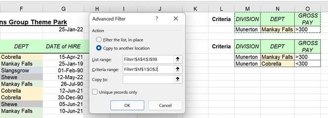
Figure 9.19 – Advanced Filter dialog box showing Criteria range selection on the worksheet
- Click inside the Copy to field, then select cell A1 to specify where you would like the filter results to appear:
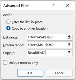
Figure 9.20 – Advanced Filter options
- Click the OK button to commit and generate the results.
- The results will appear in cell A1 of the Result worksheet:
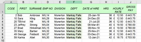
Figure 9.21 – Filter results
- Now, let’s try the OR operator criteria.
- Click inside cell A15 of the Result worksheet. Repeat the process, as per the previous filter, starting with Data | Advanced, making sure to set Criteria range to M4:O6. Lastly, select A15 in the Copy to field.
- Click OK to see the result of the filter:
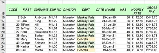
Figure 9.22 – Result of the second filter
-
Notice that the results contain all the headings from the worksheet in the result. But what if we only wanted certain columns to be represented in our result? This can be achieved by specifying this in the Copy to range. Let’s learn how to do this.
-
In the Results worksheet, we only want the Surname, Dept, and Gross Pay fields to be represented in the result. Copy the relevant fields from the Filter worksheet and paste these into cell A28 of the Result worksheet:
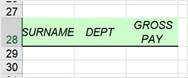
Figure 9.23 – Fields copied from the source worksheet to generate results
-
Click on a blank cell outside of the range, then navigate to Data | Advanced and fill in the fields as you did previously, except for the final step. Click inside the Copy
to field, then select cells A28:C28 to define the columns you want to generate only, based on your criteria range.
- Click OK to view the results:
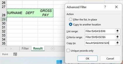
Figure 9.24 – Copy to: range A28:C28
- The result only displays the columns that have been specified according to the selected criteria:
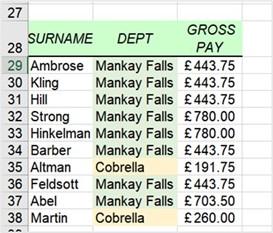
Figure 9.25 – Filter result
With that, you have learned how to use Advanced Filter and specify a unique set of columns according to set criteria as the output. Let’s investigate a few different scenarios where we will use other operators.