Conditional formatting functions
Conditional formatting is a format, such as a cell shading or font color, that’s automatically applied to cells if a specific condition is met (true). When the condition is met, a specific cell format is applied to the cells to answer any queries you may have about your data. Finding duplicate worksheet data is another great use of this tool.
In this section, you will learn how to create colored lines across workbook data when certain conditions have been met. We will be using the following validation rules and colors:
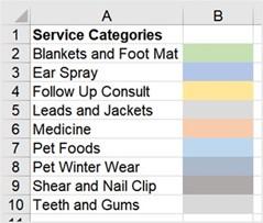
Figure 9.36 – Representation of Service Categories
We will cover the following two skills:
- The first is to set up a validation rule to make sure that data entered into a specific column on the worksheet is constrained to certain values. This is a great feature to include in the workbook when you’re working collaboratively as it ensures that if any other data is entered by a user, it is not accepted in the cell.
-
Using the conditional formatting tool based on a formula so that when a condition is met, the relevant color is applied to the row based on the selected item from the data validation drop-down list.

Setting up a validation rule
If you prefer to have a set of rules to select data from within a certain column of your workbook, you must set up a validation rule.
- Open the workbook named SSGPetFormat.xlsx to follow along.
- Let’s assume the data you are working with is on Sheet 1.
- Click the New sheet + button to create a new sheet. On Sheet 2, type the different service categories underneath each other, exactly as shown in the preceding screenshot (omitting the color codes for now).
-
To pull through the different service categories from Sheet 2 into column G on
Sheet 1, we need to set up a validation rule on Sheet 1.
- Select column L on Sheet 1.
- Click on Data | Data Validation…:
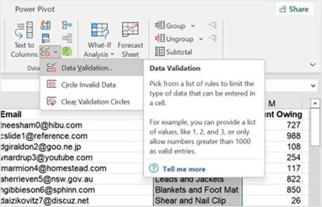
Figure 9.37 – Selecting column L, then clicking the Data Validation… button
- From the Allow field list, select List.
- Click inside the Source field, then select the arrow button to the right of the field.
- Navigate to Sheet 2 of the workbook, then select the range of criteria to include a drop-down list of categories for column L of Sheet 1:
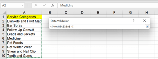
Figure 9.38 – Selecting various service categories on Sheet 2
- Click the down arrow button, then click the OK button to confirm the range you’ve selected.
- The rule will be applied to column L. You can now make selections for each cell using the drop-down list:
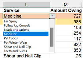
Figure 9.39 – Drop-down validation rule list